Proceedings of the 2nd Workshop on Deep Learning Approaches for Low-Resource NLP (DeepLo), pages 143–152 143
Metric Learning for Dynamic Text Classification
Jeremy Wohlwend Ethan R. Elenberg Samuel Altschul Shawn Henry Tao Lei ASAPP, Inc.
{jeremy,eelenberg,saltschul,shawn,tao}@asapp.com
Abstract
Traditional text classifiers are limited to pre-dicting over a fixed set of labels. However, in many real-world applications the label set is frequently changing. For example, in intent classification, new intents may be added over time while others are removed.
We propose to address the problem of dy-namic text classification by replacing the tra-ditional, fixed-size output layer with a learned, semantically meaningful metric space. Here the distances between textual inputs are opti-mized to perform nearest-neighbor classifica-tion across overlapping label sets. Changing the label set does not involve removing pa-rameters, but rather simply adding or remov-ing support points in the metric space. Then the learned metric can be fine-tuned with only a few additional training examples.
We demonstrate that this simple strategy is ro-bust to changes in the label space. Further-more, our results show that learning a non-Euclidean metric can improve performance in the low data regime, suggesting that fur-ther work on metric spaces may benefit low-resource research.
1 Introduction
Text classification often assumes a static set of la-bels. While this assumption holds for tasks such as sentiment analysis and part-of-speech tagging (Pang and Lee, 2005; Kim, 2014; Brants, 2000;
Collins,2002;Toutanova et al.,2003), it is rarely true for real-world applications. Consider the ex-ample of news categorization in Figure1 (a). A domain expert may decide that the Sports class should be separated into two distinct Soccer and Baseball sub-classes, and conversely merge the two Cars and Motorcycles classes into a single Auto category. Another example is user intent classification in task-oriented dialog systems. In
Sports
Cars Soccer
Baseball
Auto
Motorcycles
Place_order
Order_status
Apply_free_shipping
Redeem_$20_discount …
+
[image:1.595.314.518.220.371.2](a) news topics: (b) user intents:
Figure 1: Examples of dynamic classification. In the hierarchical setting (left), new labels are created by splitting and merging old labels. In the flat setting (right), arbitrary labels can be added or removed.
Figure1(b) for example, an intent to redeem a re-ward can be removed when the option is no longer available, while a new intent to apply free ship-ping can be added to the system. In all of these applications, the classifier must remain applicable fordynamic classification, a task where the label set is rapidly evolving.
Several factors make the dynamic classification problem difficult. First, traditional classifiers are not suited to changes in the label space. These classifiers produce a fixed sized output which aligns each of the dimensions to an existing la-bel. Thus, adding or removing any label requires changing the model architecture. Second, while it is possible to retain some model parameters, such as in hierarchical classification models, these ar-chitectures must still learn separate weights for every new class or sub-class (Cai and Hofmann,
infor-mation across similar labels, which weakens their ability to adapt to new target labels (Kowsari et al.,
2017; Tsochantaridis et al., 2005; Cai and Hof-mann,2004).
We propose to address these issues by learning an embedding function which maps input text into a semantically meaningful metric space. The pa-rameterized metric space, once trained on an ini-tial set of labeled data, can be used to perform clas-sification in a nearest-neighbor fashion (by com-paring the distance from the input text to reference texts with known label). As a result, the classifier becomes agnostic to changes in the label set. One remaining design challenge, however, is to learn a representation that best leverages the relationship between old and new labels. In particular, the la-bel split example in Figure1 (b) shows that new labels are often formed by partitioning an old la-bel. This suggests that the classifier may bene-fit from a metric space that can better represent the structural relationships between labels. Given the hierarchical relationship between the old and new labels, we choose a space of negative curva-ture (hyperbolic), which has been shown to better embed tree-like structure (Nickel and Kiela,2017;
Sala et al.,2018;Gu et al.,2019).
Our two main contributions are outlined below:
1. We design an experimental framework for dy-namic text classification, and propose a clas-sification strategy based on prototypical net-works, a simple but powerful metric learning technique (Snell et al.,2017).
2. We construct a novel prototypical network adapted to hyperbolic geometry. This re-quires deriving useful prototypes to represent a set of points on the negatively curved Rie-mannian manifold. We state sufficient theo-retical conditions for the resulting optimiza-tion problem to converge. To the best of our knowledge, this is the first application of hy-perbolic geometry to text classification be-yond the word level.
We perform a thorough experimental analysis by considering the model improvements across several aspects – low-resource fine-tuning, impact of pretraining, and ability to learn new classes. We find that the metric learning approach adapts more gracefully to changes in the label distribu-tion, and outperforms traditional, fixed size clas-sifiers in every aspect of the analysis.
Further-more, our proposed hyperbolic prototypical net-work outperforms its Euclidean counterpart in the low-resource setting, when fewer than 10 exam-ples per class are available.
2 Related Work
Prototypical Networks and Manifold Learning:
This paper builds on the prototypical network ar-chitecture (Snell et al., 2017), which was origi-nally proposed in the context of few-shot learning. In both their work and ours, the goal is to embed training data in a space such that the distance to prototypecentroids of points with the same label define good decision boundaries for labeling test data with a nearest neighbor classifier. Building on earlier work in metric learning (Vinyals et al.,
2016; Ravi and Larochelle, 2017), the authors show that learned prototype points also help the network classify inputs into test classes for which minimal data exists. This architecture has found success in computer vision applications such as image and video classification (Weinberger and Saul, 2009; Ustinova and Lempitsky, 2016; Luo et al.,2017). Very recently, prototypical network architectures have shown promising results on re-lational classification tasks (Han et al.,2018;Gao et al., 2019). To the best of our knowledge, our work is the first application of prototypical net-work architectures to text classification using non-Euclidean geometry.1
Concurrent with the writing of this paper, (Khrulkov et al.,2019) applied several hyperbolic neural networks to few-shot image classification tasks. However, their prototypical network uses the Einstein midpoint rather than the Karcher mean we use in Section3.3. In (Chen et al.,2019) the authors embed the labels and data separately, then predict hierarchical class membership using an interaction model. Our model directly links embedding distances to model predictions, and thus learns an embedded space that is more amenable to low-resource, dynamic classification tasks.
Hyperbolic geometry has been deeply ex-plored in classical works of differential geome-try (Thurston,2002;Cannon et al.,1997;Berger,
2003). More recently, hyperbolic space has been studied in the context of developing neural net-works with hyperbolic parameters (Ganea et al.,
2018b). In particular, recent work has success-fully applied hyperbolic geometry to graph em-beddings (Sarkar, 2011;Nickel and Kiela, 2017,
2018;Sala et al., 2018; Ganea et al., 2018a;Gu et al., 2019). In all of these prior works, the model’s parameters correspond to node vectors in hyperbolic space that require Riemannian op-timization. In our case, only the model’s out-puts live in hyperbolic space—not its parameters, which avoids propagating gradients in hyperbolic space and facilitates optimization. This is ex-plained in more detail in Section3.3.
Hierarchical or Few-shot Text Classification:
Many classical models for multi-class classi-fication incorporate a hierarchical label struc-ture (Tsochantaridis et al., 2005; Cai and Hof-mann, 2004; Yen et al., 2016;Naik et al., 2013;
Sinha et al., 2018). Most models proceed in a top-down manner: a separate classifier (logistic re-gression, SVM, etc.) is trained to predict the cor-rect child label at each node in the label hierarchy. For instance, HDLTex (Kowsari et al., 2017) ad-dresses large hierarchical label sets explicitly by training a stacked, hierarchical neural network ar-chitecture. Such approaches do not scale well to deep and large label hierarchies, while our method can adapt to more flexible settings, such as adding or removing labels, without adding extra parame-ters.
Our work also relates to text classification in a low-resource setting. While a wide range of meth-ods improve accuracy by leveraging external data such as multi-task training (Miyato et al., 2016;
Chen et al.,2018;Yu et al.,2018;Guo et al.,2018), semi-supervised pretraining (Dai and Le, 2015), and unsupervised pretraining (Peters et al.,2018;
Devlin et al.,2018), our method makes use of the structure of the data via metric learning. As a re-sult, our method can be easily combined with any of these methods to further improve model perfor-mance.
3 Model Framework
This section provides the details of each compo-nent of our framework, starting with a more de-tailed formulation ofdynamic classification. We then provide some background on prototypical
networks, before introducing our hyperbolic vari-ant and its theoretical guarvari-antees.
3.1 Dynamic Classification
Mathematically, we formulatedynamic classifica-tion as the following problem: given access to an old, labeled training corpus(xi, yi) 2 Xold⇥ Yold, we are interested in training a classifier h: Xnew 7! Ynew with a few examples (xj, yj) 2 Xnew⇥Ynew. Unlike few-shot learning, the old
and new datasets need not be disjoint (Xold \ Xnew6=;,Yold\Ynew6=;).
We consider two different cases: 1) new la-bels arrive as a consequence of new input data
Xnew\ Xold, and 2) during label splitting/merging,
some new examples may be constructed by re-labeling old examples from yi 2 Yold to yj 2 Ynew \ Yold. This latter case is of particular
in-terest as the classifier may be able to leverage its knowledge of old labels in learning to classify new ones.
There are many natural approaches to this prob-lem. First, a fixed model trained on Xold⇥Yold
may be applied directly to classify examples in
Xnew⇥Ynew, which we refer to as anun-tuned
model. Alternately, a pretrained model may also be fine-tuned onXnew⇥Ynew. Finally, it is also
possible to train from scratch on Xnew ⇥Ynew,
disregarding the model weights trained on the old data distribution. We compare strategies in Sec-tions4–5.
3.2 Episodic Training
The standard prototypical network is trained us-ing episodic trainus-ing, as described in (Snell et al.,
2017). We view our model as an embedding func-tion which takes textual inputs and outputs points in the metric space. Let d(x, y) denote the
dis-tance between two points x and y in our metric space, and let f denote our embedding function. At each iteration, we form a new episode by sam-pling a set of target labels, as well as support and query points for each of the sampled labels. Let NC,NS, andNQ, be the number of classes tested,
the number of support points used, and the number of query points used in each episode, respectively. For each episode, we first sample NC classes,
C = {ci|i = 1, . . . , NC}, uniformly across all
training labels. We then build a set of support points Si = {si,j|j = 1, . . . , NS} for each of
the selected classes by samplingNS training
set, we compute a prototype vector p⇤i. For the standard Euclidean prototypical network, we use the mean of the embedded support set:
p⇤i = 1
NS NS
X
j=1
f(si,j) . (1)
To compute the loss for an episode, we fur-ther sample NQ query points Q = {xi,j|j =
1, . . . , NQ} which do not appear in the support
set of the episode, for each selected classci. We
then encode each query sequence and apply a soft-max function over the negative distances from the query points to the episode’s class prototypes. This yields a probability distribution over classes, and we take the negative log probability of the true class, averaged over the query points, to get the loss for the episode.
1
NCNQ NC
X
i=1
NQ
X
j=1
log
exp( d(f(xi,j), p⇤i)) P
kexp( d(f(xi,j), p⇤k))
,
wherekin the denominator ranges from1toNC.
The steps of a single episode are summarized in Algorithm1.
Once episodic training is finished, the prototype vectors for a class can be computed as the mean of the embeddings of any number of items in the class. In our experiments, we use the whole train-ing set to compute the final class prototypes, but under lower resources, fewer support points could also be used.
3.3 Hyperbolic Prototypical Networks
In this section we discuss the hyperbolic prototyp-ical network which can better model structural re-lationships between labels. We first review the hy-perboloid model of hyperbolic space and its dis-tance formula. Then we describe the main tech-nical challenge of computing good prototypes in hyperbolic space. Proofs of our uniqueness and convergence will be provided in an extended ver-sion. We also describe a second, distinctmethod for computing prototypes which is used to initial-ize our main method during experiments (a de-tailed discussion of this point will be provided in an extended version).
Hyperbolic space can be interpreted as a con-tinuous analogue of a tree (Cannon et al., 1997;
Krioukov et al., 2010). While trees on n ver-tices can be embedded in Euclidean space with
log(n) dimensions, hyperbolic space needs only
Algorithm 1Prototypical Training Episode
Input:D– set of(x, y)pairs
Di – all pairs withy =i
NC – number of classes sampled each episode
NS– number of support points
NQ– number of query points
1: procedureEPISODE(D,NC,NS,NQ)
2: C SAMPLE(D, NC)
3: fori2Cdo
4: Si SAMPLE(Di, NS)
5: Qi SAMPLE(Di\Si, NQ)
6: ci PROTOTYPE(Si)
7: P CONCAT(c0;c1; ...;cNC)
8: Loss 0
9: for eachQido
10: di PAIRWISEDIST(Qi, P)
11: Loss Loss N 1
CNQlog
e di
P
je dj
2 dimensions. Additionally, the circumference of a hyperbolic disk grows exponentially with its ra-dius. Therefore, hyperbolic models have room to place many prototypes equidistant from a common parent while maintaining separability from other classes. We argue that this property helps text clas-sification with latent hierarchical structures (e.g. dynamic label splitting).
The reader is referred to Section 2.6 of (Thurston, 2002) for a detailed introduc-tion to hyperbolic geometry, and to (Cannon et al., 1997) for a more gentle introduction. In this section we have adopted the sign convention of (Sala et al.,2018).
Hyperbolic space inddimensions is the unique, simply connected, d-dimensional, Riemannian manifold with constant curvature 1. The
hyper-boloid (or Lorentz) model realizesd-dimensional hyperbolic space as an isometric embedding in-side Rd+1 endowed with a signature(1, d) bilin-ear form. Specifically, let the coordinates of any a 2 Rd+1 be a = (a
0, a1, ..., ad). Then we can
define a bilinear form onRd+1by
B(x, y) =x0y0
d X
j=1
which allows us to define the hyperboloid to be the set{x 2Rd+1|B(x, x) = 1andx0 >0}. We induce a Riemannian metric on the hyperboloid by restrictingB(·,·) to the hyperboloid’s tangent space. The resulting Riemannian manifold is hy-perbolic spaceHd. Forx, y 2 Hd the hyperbolic
distance is given by
dH(x, y) = arccosh(B(x, y)). (3)
There are several equivalent ways of defining hyperbolic space. We choose to work primarily in the hyperboloid model over other models (e.g. Poincar´e disk model) for improved numerical sta-bility. We use the d-dimensional output vectorh of our network and project it on the hyperboloid embedded ind+ 1dimensions:
h0 =
v u u
tXd
i=1 h2
i + 1 , h¯= [h0;h] . (4)
A key algorithmic difference between the Eu-clidean and the hyperbolic model is the computa-tion of prototype vectors. There are multiple defi-nitions that generalize the notion of a mean to gen-eral Riemannian manifolds. One sensible mean p?X of a set X is given by the point which mini-mizes the sum of squared distances to each point inX.
p?X = arg min
p2Hd X
(p)
= arg min
p2Hd
X
x2X
dHd(p, x)2 .
(5)
A proof for the following proposition will be pro-vided in an extended version. We note that concur-rent with the writing of this paper, a generalized version of our result appeared in (Gu et al.,2019) as Lemma 2.
Proposition 1. Every finite collection of pointsX inHdhas a unique meanp?
X. Furthermore,
solv-ing the optimization problem(5)with Riemannian gradient descent will converge top?
X.
In an effort to derive a closed form for p?X (rather than solve a Riemannian optimization problem), we conjecture that the following expres-sion is a good approximation. It is computed by averaging the vectors in X and scaling them by the constant which projects this average back to the hyperboloid:
ˆ
p= 1
|X|
X
x2X
x, p˜= p pˆ
B(ˆp,pˆ). (6)
p?
X 6= ˜p can be shown to differ through a
sim-ple counterexamsim-ple, although in practice we find little difference between their values during exper-iments. The proof will be provided in an extended version.
3.4 Implementation and Stability
Our final hyperbolic prototypical model combines both definitions with the following heuristic: ini-tialize problem (5) withp˜and then run several
it-erations of Riemannian gradient descent. We find that it is possible to backpropagate through a few steps of the gradient descent procedure described above during prototypical model training. How-ever, we also find that the model can be trained successfully when detaching the gradients with re-spect to the support points. This suggests that pro-totypical models can be trained in metric spaces where the mean or its gradient cannot be computed efficiently. Further experimental details are pro-vided in the next section.
Our prototypical network loss function uses both squared Euclidean distance and squared hy-perbolic distance for similar reasons. Namely, the distance between two close points is much less nu-merically stable than the squared distance. In the Euclidean case, the derivative ofpsis undefined at zero. In the hyperbolic case, the derivative of
arccosh(s)at1is undefined, andB(x, x) = 1for
points on the hyperboloid. If we instead use the squaredhyperbolic distance, L’Hˆopital’s rule im-plies that the derivative ofarccosh(b)2asb!1+ is2, allowing gradients to backpropagate through the squared hyperbolic distance without issue.
4 Experiments
We evaluate the performance of our framework on several text classification benchmarks, two of which exhibit a hierarchical label set. We only use the label hierarchy to simulate the label split-ting discussed in Figure 1 (a). The models are not trained with explicit knowledge of the hierarchy, as we assume that the full hierarchy is not known a priori in the dynamic classification setting. A description of the datasets is provided below:
• 20 Newsgroups (NEWS): This dataset is composed of nearly 20,000 documents, dis-tributed across 20 news categories. We use the provided label hierarchy to form the depth
use 9,044 documents for training, 2,668 for validation, and 7,531 for testing.
• Web of Science (WOS): This dataset was used in two previous works on hierarchical text classification (Kowsari et al.,2017;Sinha et al., 2018). It contains 134 topics, split across 7 parent categories. It contains 46,985 documents collected from the Web of Science citation index. We use 25,182 documents for training, 6,295 for validation, and 15,503 for testing.
• Twitter Airline Sentiment (SENT): This
dataset consists of public tweets from cus-tomers to American-based airlines labeled with one of10reasons for negative sentiment
(e.g. Late Flight, Lost Luggage).2 We pre-process the data by keeping only the nega-tive tweets with confidence over 60%. This
dataset is non-hierarchical and composed of nearly 7500 documents. We use 5,975 doc-uments for training, 742 for validation, and 754 for testing.
Dynamic Setup: We construct training data for the task of dynamic classification as follows. First, we split our training data in half. The first half is used for pretraining and the second for fine-tuning. To simulate a change in the label space, we ran-domly removep > 0fraction of labels in the
pre-training data. This procedure yields two label sets, with Yold (pretraining)⇢ Ynew (fine-tuning). In
our experiments, we further vary the amount of data available in the fine-tuning set. For the flat dataset, the labels to be removed are sampled uni-formly. In the hierarchical case, we createYoldby
randomly collapsing leaf labels into their parent classes, as shown previously in Figure1.
Hyperparameters and Implementation Details:
We apply the same encoder architecture through-out all experiments. We use a 4 layer recurrent neural network, with SRU cells (Lei et al.,2018) and a hidden size of 128. We use pretrained GloVe embeddings (Pennington et al.,2014), which are fixed during training. A sequence level embedding is computed by passing a sequence of word em-beddings through the recurrent encoder, and tak-ing the embeddtak-ing for the last token to represent
2https://www.kaggle.com/crowdflower/
twitter-airline-sentiment
the sequence. We use the ADAM optimizer with default learning of 0.001, and train for 100 epochs for the baseline models and 10,000 episodes for the prototypical models, with early stopping. In our experiments, we useNS = 4,NQ = 64. We
use the full label set every episode for all datasets except WOS, for which we useNC = 50. We use
a dropout rate of 0.5 on NEWS and SENT, and 0.3 for the larger WOS dataset. We tuned the learn-ing rate and dropout for each model on a held-out validation set.
For the hyperbolic prototypical network, we fol-low the initialization and update procedure out-lined at the end of Section3.3with5iterations of
Riemannian gradient descent during training and
100iterations during evaluation. We utilize
neg-ative squared distance in the softmax computa-tion in order to improve numerical stability. The means are computed via (5) during both training and model inference. However, this computation is treated as a constant during backpropagation as described in Section3.3.
Baseline: Our baseline model consists of the same recurrent encoder and an extra linear output layer which computes the final probabilities over the target classes. In order to fine-tune this multi-layer perceptron (MLP) model on a new label on-tology, we reuse the encoder, and learn a new out-put layer. This differs from the prototypical mod-els for which the architecture is kept unchanged.
Evaluation: We evaluate the performance of our models using accuracy with respect to the new label set Ynew. We also highlight accuracy on
only the classes introduced during label addi-tion/splitting,i.e. Ynew\ Yold. All results are
av-eraged over5random label splits withp= 0.3.
Results: Table1shows the accuracy of the fine tuned models for all three methods. The SENT dataset shows performance in the case where com-pletely new labels are added during fine tuning. In the NEWS and WOS datasets new labels originate from the splits of old labels.
In all cases, the prototypical models outperform the baseline MLP model significantly, especially when the data in the new label distribution is in the low-resource regime (+5–15% accuracy). We also see an increase in performance in the high data regime of up to 5%.
Dataset Model nf ine= 5 nf ine= 10 nf ine= 20 nf ine= 100
MLP 37.3±2.9 43.8±3.5 45.7±3.8 57.4±3.5
SENT EUC 39.6±6.4 45.5±1.8 47.7±4.7 62.7±2.1
HYP 42.2±3.5 47.1±4.8 53.0±2.3 62.7±2.2
MLP 49.2±1.0 55.9±2.5 68.5±1.1 76.3±0.5
NEWS EUC 56.5±0.4 65.6±1.0 74.2±0.6 79.8±0.2
HYP 64.8±2.8 69.7±1.0 72.9±0.5 78.8±0.4
MLP 36.6±1.1 46.8±1.2 62.8±0.6 68.9±0.5
WOS EUC 49.4±1.0 59.2±0.4 70.4±0.4 73.3±0.2
[image:7.595.129.470.62.201.2]HYP 54.5±1.4 60.7±0.9 70.2±0.7 73.5±0.5
Table 1: Test accuracy for each dataset and method. Columns indicate the number of examples per labelnf ine used in the fine tuning stage. In all cases, the prototypical models outperform the baseline. The hyperbolic model performs best in the low data regime, but both metrics perform comparably when data is abundant.
data regime on the NEWS and WOS datasets. This is consistent with our hypothesis (and previ-ous work) that hyperbolic geometry is well suited for hierarchical data. Interestingly, the hyperbolic model also performs better on the non-hierarchical SENT dataset when given few examples, which implies that certain metric spaces may be gener-ally stronger in the low-resource setting. In the high data regime, however, both prototypical mod-els perform comparably.
5 Analysis
In this section, we examine several aspects of our experimental setup more closely, and use the SENT and NEWS datasets for this analysis.
Benefits of Pretraining We wish to isolate the effect of pretraining on an older label set by mea-suring the performance of our models on the new label distribution with and without pretraining. Figure 2 shows accuracy without pretraining as solid bars, with the gains due to pretraining shown as translucent bars above them. In the low-data regime without pretraining, all models often per-form similarly. Nevertheless, our models do im-prove substantially over the baseline once pre-training is introduced.
With only a few new examples, our models bet-ter leverage knowledge gained from old pretrain-ing data. On the NEWS dataset in particular, with only 5 fine-tune examples per class, the relative re-duction in classification error for metric learning models exceeds 53% (Euclidean) and 62%
(hy-perbolic), while the baseline only reduces relative error by about 45%. This shows that the
proto-typical network, and particularly the hyperbolic
5 10 20 100
0.0 0.2 0.4 0.6 0.8 1.0
Accuracy
MLP Euclidean Hyperbolic
(a) SENT
5 10 50 500
0.0 0.2 0.4 0.6 0.8 1.0
Accuracy
MLP Euclidean Hyperbolic
(b) NEWS
Figure 2: Accuracy gains from pretraining as a func-tion of the number of examples per class available in the new label distribution. While the models are com-parable in the pretraining stage (solid bards), the proto-typical models make better use of pretraining, showing higher gain during fine-tuning in both the low and high data data regimes (translucent bars).
model can adapt more quickly to dynamic label shifts. Furthermore, the prototypical models con-serve their advantage over the baseline in the high data regime, though the margins become smaller.
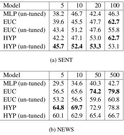
[image:7.595.309.522.271.506.2]per-Model 5 10 20 100 MLP (un-tuned) 38.2 46.7 42.4 46.3 EUC 39.6 45.5 47.7 62.7
EUC (un-tuned) 43.4 51.2 47.6 55.8 HYP 42.2 47.1 53.0 62.7
HYP (un-tuned) 45.7 52.4 53.3 53.1
(a) SENT
Model 5 10 50 500
MLP (un-tuned) 29.5 34.6 40.3 42.7 EUC 56.5 65.6 74.2 79.8
EUC (un-tuned) 53.2 56.5 59.6 60.8 HYP 64.8 69.7 72.9 78.8 HYP (un-tuned) 60.1 62.9 65.4 66.7
[image:8.595.78.286.60.286.2](b) NEWS
Table 2: Test accuracy for each dataset and method. Columns indicate the number of examples per label used for fine-tuning and/or creating prototype vectors.
formance, or whether fine-tuning should only be done once a significant amount of data has been obtained from the new distribution. We study this question by comparing the performance of tuned and un-tuned models on the new label distribution. Table 2 compares the accuracy of two types of pretrained prototypical models provided with a variable number of new examples. The fine-tuned model uses this data for both additional training and for constructing new prototypes. The un-tuned model constructs prototypes using the pretrained model’s representations without addi-tional training. We also construct an un-tuned MLP baseline by fitting a nearest neighbor clas-sifier (KNN) on the encodings of the penultimate layer of the network. We experimented with fitting the KNN on the output predictions but found that using the penultimate layer was more effective.
We find that the models generally benefit from fine-tuning once a significant amount of data for the new classes is provided (>20). In the low data regime, however, the results are less consistent, and suggests that the performance may be very dataset dependant. We note however that all met-ric learning models significantly outperform the MLP-KNN baseline in both the low and high data regimes. This shows that regardless of fine-tuning, our approach is more robust on previously unseen classes.
5 10 50 500
0.0 0.2 0.4 0.6 0.8 1.0
Accuracy
MLP Euclidean Hyperbolic
(a) Accuracy with respect to the full label set
5 10 50 500
0.0 0.2 0.4 0.6 0.8 1.0
Accuracy (new)
MLP Euclidean Hyperbolic
[image:8.595.317.512.61.265.2](b) Accuracy with respect to new classes only
Figure 3: Accuracy on the NEWS Dataset against num-ber of fine tune examples: (a) all classes and (b) newly introduced classes only. The mean is taken over 5 ran-dom label splits, and error bars are given at±1standard
deviation. The gap between the hyperbolic models and the others is even larger on the new classes.
Learning New Classes An important factor in the dynamic classification setup is the ability for the model to not only keep performing well on the old classes, but also to smoothly adapt to new ones. We highlight the performance of the models on the newly introduced labels in Figure3, where we see that the improvement in accuracy is domi-nated by the performance on the new classes.
6 Conclusions
References
Marcel Berger. 2003. A Panoramic View of Rieman-nian Geometry. Springer-Verlag Berlin Heidelberg, Heidelberg, Germany.
Thorsten Brants. 2000. Tnt: a statistical part-of-speech tagger. In Proceedings of the sixth conference on Applied natural language processing, pages 224– 231. Association for Computational Linguistics.
Lijuan Cai and Thomas Hofmann. 2004. Hierarchi-cal document categorization with support vector ma-chines. InCKIM, pages 78–87.
James Cannon, William Floyd, Richard Kenyon, and Walter Parry. 1997. Hyperbolic
geome-try. http://library.msri.org/books/
Book31/files/cannon.pdf.
Boli Chen, Xin Huang, Lin Xiao, Zixin Cai, and Lip-ing JLip-ing. 2019. Hyperbolic interaction model for hierarchical multi-label classification. https://
arxiv.org/pdf/1905.10802.pdf.
Xilun Chen, Yu Sun, Ben Athiwaratkun, Claire Cardie, and Kilian Weinberger. 2018. Adversarial deep av-eraging networks for cross-lingual sentiment classi-fication. Transactions of the Association for Com-putational Linguistics, 6.
Michael Collins. 2002. Discriminative training meth-ods for hidden markov models: Theory and ex-periments with perceptron algorithms. In EMNLP, pages 1–8. Association for Computational Linguis-tics.
Andrew M Dai and Quoc V Le. 2015. Semi-supervised sequence learning. InNeurIPS, pages 3079–3087.
Jacob Devlin, Ming-Wei Chang, Kenton Lee, and Kristina Toutanova. 2018. Bert: Pre-training of deep bidirectional transformers for language understand-ing. InNAACL.
Octavian-Eugen Ganea, Gary B´ecigneul, and Thomas Hofmann. 2018a. Hyperbolic entailment cones for learning hierarchical embeddings. InICML.
Octavian-Eugen Ganea, Gary B´ecigneul, and Thomas Hofmann. 2018b. Hyperbolic neural networks. In NeurIPS.
Tianyu Gao, Xu Han, Zhiyuan Liu, and Maosong Sun. 2019. Hybrid attention-based prototypical networks for noisy few-shot relation classification. InAAAI.
Albert Gu, Frederic Sala, Beliz Gunel, and Christopher R´e. 2019. Learning mixed-curvature representations in products of model spaces. InICLR.
Jiang Guo, Darsh Shah, and Regina Barzilay. 2018. Multi-source domain adaptation with mixture of ex-perts. In EMNLP. Association for Computational Linguistics.
Xu Han, Hao Zhu, Pengfei Yu, Ziyun Wang, Yuan Yao, Zhiyuan Liu, and Maosong Sun. 2018. Fewrel: A large-scale supervised few-shot relation classifi-cation dataset with state-of-the-art evaluation. In EMNLP.
Valentin Khrulkov, Leyla Mirvakhabova, Evgeniya Ustinova, Ivan Oseledets, and Victor Lempitsky. 2019. Hyperbolic image embeddings. https:
//arxiv.org/pdf/1904.02239.pdf.
Yoon Kim. 2014. Convolutional neural networks for sentence classification. InEMNLP, page 17461751. Kamran Kowsari, Donald E. Brown, Mojtaba Hei-darysafa, Kiana Jafari Meimandi, Matthew S. Ger-ber, and Laura E. Barnes. 2017. HDLTex: hierar-chical deep learning for text classification. InIEEE ICMLA, pages 364–371.
Dmitri Krioukov, Fragkiskos Papadopoulos, Maksim Kitsak, Amin Vahdat, and Mari´an Bogu˜n´a. 2010. Hyperbolic geometry of complex networks. Phys. Rev. E, 82.
Tao Lei, Yu Zhang, Sida I. Wang, Hui Dai, and Yoav Artzi. 2018. Simple recurrent units for highly paral-lelizable recurrence. InEMNLP.
Zelun Luo, Yuliang Zou, Judy Hoffman, and Li Fei-Fei. 2017. Label efficient learning of transfer-able representations across domains and tasks. In NeurIPS.
Takeru Miyato, Andrew M Dai, and Ian Good-fellow. 2016. Adversarial training methods for semi-supervised text classification. arXiv preprint arXiv:1605.07725.
Azad Naik, Anveshi Charuvaka, and Huzefa Rangwala. 2013. Classifying documents within multiple hier-archical datasets using multi-task learning. InIEEE International Conference on Tools with Artificial In-telligence.
Maximilian Nickel and Douwe Kiela. 2018. Learning continuous hierarchies in the lorentz model of hy-perbolic geometry. InICML, pages 3776–3785. Maximillian Nickel and Douwe Kiela. 2017. Poincar´e
embeddings for learning hierarchical representa-tions. InNeurIPS, pages 6338–6347.
Bo Pang and Lillian Lee. 2005. Seeing stars: Exploit-ing class relationships for sentiment categorization with respect to rating scales. InProceedings of the annual meeting on assocation for computational lin-gustics, pages 115–224.
Sachin Ravi and Hugo Larochelle. 2017. Optimization as a model for few-shot learning. InICLR.
Frederic Sala, Chris De Sa, Albert Gu, and Christopher R´e. 2018. Representation tradeoffs for hyperbolic embeddings. InICML, pages 4460–4469.
R. Sarkar. 2011. Low distortion Delaunay embedding of trees in hyperbolic plane. InProc. of the Inter-national Symposium on Graph Drawing (GD 2011), pages 355–366.
Koustuv Sinha, Yue Dong, Jackie Chi Kit Cheung, and Derek Ruths. 2018. A hierarchical neural attention-based text classifier. InEMNLP, pages 817–823.
Jake Snell, Kevin Swersky, and Richard Zemel. 2017. Prototypical networks for few-shot learning. In NeurIPS, pages 4077–4087.
William Thurston. 2002. The geometry and topol-ogy of three-manifolds: Chapter 2, elliptic and hy-perbolic geometry. http://library.msri.
org/books/gt3m/PDF/2.pdf.
Kristina Toutanova, Dan Klein, Christopher D Man-ning, and Yoram Singer. 2003. Feature-rich part-of-speech tagging with a cyclic dependency network. InNAACL, pages 173–180. Association for Compu-tational Linguistics.
Ioannis Tsochantaridis, Thorsten Joachims, Thomas Hofmann, and Yasemin Altun. 2005. Large mar-gin methods for structured and interdependent out-put variables. JMLR, 6:1453–1484.
Evgeniya Ustinova and Victor Lempitsky. 2016. Learning deep embeddings with histogram loss. In NeurIPS, pages 4170–4178.
Oriol Vinyals, Charles Blundell, Timothy Lillicrap, Koray Kavukcuoglu, and Daan Wierstra. 2016. Matching networks for one shot learning. In NeurIPS, pages 3630–3638.
Kilian Weinberger and Lawrence Saul. 2009. Dis-tance metric learning for large margin nearest neigh-bor classification. Journal of Machine Learning Re-search, 10:207–244.
Ian En-Hsu Yen, Xiangru Huang, Pradeep Ravikumar, Kai Zhong, and Inderjit Dhillon. 2016. Pd-sparse: A primal and dual sparse approach to extreme mul-ticlass and multilabel classification. InICML, pages 3069–3077.
Mo Yu, Xiaoxiao Guo, Jinfeng Yi, Shiyu Chang, Saloni Potdar, Yu Cheng, Gerald Tesauro, Haoyu Wang, and Bowen Zhou. 2018. Diverse few-shot text clas-sification with multiple metrics. InNAACL.