Analysis of Stopping Active Learning based on Stabilizing Predictions
Michael Bloodgood
Center for Advanced Study of Language University of Maryland
College Park, MD 20740
John Grothendieck
Raytheon BBN Technologies 9861 Broken Land Parkway, Suite 400
Columbia, MD 21046
Abstract
Within the natural language processing (NLP) community, active learning has been widely investigated and applied in or-der to alleviate the annotation bottleneck faced by developers of new NLP systems and technologies. This paper presents the first theoretical analysis of stopping active learning based on stabilizing predictions (SP). The analysis has revealed three ele-ments that are central to the success of the SP method: (1) bounds on Cohen’s Kappa agreement between successively trained models impose bounds on differences in F-measure performance of the models; (2) since the stop set does not have to be la-beled, it can be made large in practice, helping to guarantee that the results trans-fer to previously unseen streams of ex-amples at test/application time; and (3) good (low variance) sample estimates of Kappa between successive models can be obtained. Proofs of relationships between the level of Kappa agreement and the dif-ference in performance between consecu-tive models are presented. Specifically, if the Kappa agreement between two mod-els exceeds a threshold T (whereT > 0),
then the difference in F-measure perfor-mance between those models is bounded above by 4(1−T)
T in all cases. If precision
of the positive conjunction of the models is assumed to bep, then the bound can be
tightened to4(1−T) (p+1)T.
1 Introduction
Active learning (AL), also called query learning
andselective sampling, is an approach to reduce the costs of creating training data that has received considerable interest (e.g., (Argamon-Engelson
and Dagan, 1999; Baldridge and Osborne, 2008; Bloodgood and Vijay-Shanker, 2009b; Bloodgood and Callison-Burch, 2010; Hachey et al., 2005; Haertel et al., 2008; Haffari and Sarkar, 2009; Hwa, 2000; Lewis and Gale, 1994; Sassano, 2002; Settles and Craven, 2008; Shen et al., 2004; Thompson et al., 1999; Tomanek et al., 2007; Zhu and Hovy, 2007)).
Within the NLP community, active learning has been widely investigated and applied in order to alleviate the annotation bottleneck faced by devel-opers of new NLP systems and technologies. The main idea is that by judiciously selecting which examples to have labeled, annotation effort will be focused on the most helpful examples and less an-notation effort will be required to achieve given levels of performance than if a passive learning policy had been used.
Historically, the problem of developing meth-ods for detecting when to stop AL was tabled for future work and the research literature was fo-cused on how to select which examples to have la-beled and analyzing the selection methods (Cohn et al., 1996; Seung et al., 1992; Freund et al., 1997; Roy and McCallum, 2001). However, to realize the savings in annotation effort that AL enables, we must have a method for knowing when to stop the annotation process. The challenge is that if we stop too early while useful generalizations are still being made, then we can wind up with a model that performs poorly, but if we stop too late after all the useful generalizations are made, then hu-man annotation effort is wasted and the benefits of using active learning are lost.
Recently research has begun to develop meth-ods for stopping AL (Schohn and Cohn, 2000; Ertekin et al., 2007b; Ertekin et al., 2007a; Zhu and Hovy, 2007; Laws and Sch¨utze, 2008; Zhu et al., 2008a; Zhu et al., 2008b; Vlachos, 2008; Bloodgood, 2009; Bloodgood and Vijay-Shanker, 2009a; Ghayoomi, 2010). The methods are all
heuristics based on estimates of model confidence, error, or stability. Although these heuristic meth-ods have appealing intuitions and have had ex-perimental success on a small handful of tasks and datasets, the methods are not widely usable in practice yet because our community’s understand-ing of the stoppunderstand-ing methods remains too coarse and inexact. Pushing forward on understanding the mechanics of stopping at a more exact level is therefore crucial for achieving the design of widely usable effective stopping criteria.
Bloodgood and Vijay-Shanker (2009a) intro-duce the terminology aggressive and conserva-tive to describe the behavior of stopping meth-ods1 and conduct an empirical evaluation of the different published stopping methods on several datasets. While most stopping methods tend to behave conservatively, stopping based on stabiliz-ing predictions computed via inter-model Kappa agreement has been shown to be consistently ag-gressive without losing performance (in terms of F-Measure2) in several published empirical tests. This method stops when the Kappa agreement be-tween consecutively learned models during AL exceeds a threshold for three consecutive itera-tions of AL. Although this is an intuitive heuristic that has performed well in published experimental results, there has not been any theoretical analysis of the method.
The current paper presents the first theoretical analysis of stopping based on stabilizing predic-tions. The analysis helps to explain at a deeper and more exact levelwhy the method works as it does. The results of the analysis help to character-ize classes of problems where the method can be expected to work well and where (unmodified) it will not be expected to work as well. The theory is suggestive of modifications to improve the ro-bustness of the stopping method for certain classes of problems. And perhaps most important, the approach that we use in our analysis provides an enabling framework for more precise analysis of stopping criteria and possibly other parts of the ac-tive learning decision space.
In addition, the information presented in this
pa-1Aggressive methods stop sooner, aggressively trying to
reduce unnecessary annotations while conservative methods are careful not to risk losing model performance, even if it means annotating many more examples than were necessary.
2For the rest of this paper, we will use F-measure to
de-note F1-measure, that is, the balanced harmonic mean of pre-cision and recall, which is a standard metric used to evaluate NLP systems.
per is useful for works that consider switching be-tween different active learning strategies and oper-ating regions such as (Baram et al., 2004; D¨onmez et al., 2007; Roth and Small, 2008). Knowing when to switch strategies, for example, is sim-ilar to the stopping problem and is another set-ting where detailed understanding of the variance of stabilization estimates and their link to perfor-mance ramifications is useful. More exact un-derstanding of the mechanics of stopping is also useful for applications of co-training (Blum and Mitchell, 1998), and agreement-based co-training (Clark et al., 2003) in particular. Finally, the proofs of the Theorems regarding the relationships between Cohen’s Kappa statistic and F-measure may be of broader use in works that consider inter-annotator agreement and its ramifications for per-formance appraisals, a topic that has been of long-standing interest in computational linguistics (Car-letta, 1996; Artstein and Poesio, 2008).
In the next section we summarize the stabiliz-ing predictions (SP) stoppstabiliz-ing method. Section 3 analyzes SP and Section 4 concludes.
2 Stopping Active Learning based on Stabilizing Predictions
The intuition behind the SP method is that the models learned during AL can be applied to a large representative set of unlabeled data called a stop set and when consecutively learned models have high agreement on their predictions for classify-ing the examples in the stop set, this indicates that it is time to stop (Bloodgood and Vijay-Shanker, 2009a; Bloodgood, 2009). The active learning stopping strategy explicitly examined in (Blood-good and Vijay-Shanker, 2009a) (after the general form is discussed) is to calculate Cohen’s Kappa agreement statistic between consecutive rounds of active learning and stop once it is above 0.99 for three consecutive calculations.
of the agreement metrics they discuss are of the form:
agreement= Ao−Ae 1−Ae
, (1)
whereAo =observed agreement, andAe =
agree-ment expected by chance. The different metrics differ in how they computeAe. All the instances
of usage of an agreement metric in this article will have two categories and two coders. The two cat-egories are “+1” and “-1” and the two coders are the two consecutive models for which agreement is being measured.
Cohen’s Kappa statistic3 (Cohen, 1960) mea-sures agreement expected by chance by modeling each coder (in our case model) with a separate dis-tribution governing their likelihood of assigning a particular category. Formally, Kappa is defined by Equation 1 withAecomputed as follows:
Ae=
X
k∈{+1,−1}
P(k|c1)·P(k|c2), (2)
where each ci is one of the coders (in our case,
models), andP(k|ci)is the probability that coder
(model)cilabels an instance as being in category k. Kappa estimates the P(k|ci) in Equation 2
based on the proportion of observed instances that coder (model)ci labeled as being in categoryk.
3 Analysis
This section analyzes the SP stopping method. Section 3.1 analyzes the variance of the estima-tor of Kappa that SP uses and in particular the re-lationship of this variance to specific aspects of the operationalization of SP, such as the stop set size. Section 3.2 analyzes relationships between the Kappa agreement between two models and the difference in F-measure between those two mod-els.
3.1 Variance of Kappa Estimator
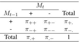
SP bases its decision to stop on the information contained in the contingency tables between the classifications of models learned at consecutive iterations during AL. In determining whether to stop at iteration t, the classifications of the current modelMtare compared with the classifications of
the previous modelMt−1. Table 1 shows the
pop-ulation parameters for these two models, where:
3We note that there are other agreement measures (beyond
Cohen’s Kappa) which could also be applicable to stopping based on stabilizing predictions, but an analysis of these is outside the scope of the current paper.
Mt
Mt−1 + - Total
+ π++ π+− π+.
- π−+ π−− π−.
[image:3.595.349.486.60.133.2]Total π.+ π.− 1
Table 1: Contingency table population probabili-ties forMt(model learned at iteration t) andMt−1
(model learned at iteration t-1).
population probabilityπij fori, j∈ {+,−}is the
probability of an example being placed in category
i by model Mt−1 and category j by model Mt;
population probability π.j for j ∈ {+,−} is the
probability of an example being placed in category
jby modelMt; and population probabilityπi.for i∈ {+,−}is the probability of an example being placed in category iby modelMt−1. The actual
probability of agreement isπo=π+++π−−. As indicated in Equation 2, Kappa models the prob-ability of agreement expected due to chance by assuming that classifications are made indepen-dently. Hence, the probability of agreement ex-pected by chance in terms of the population prob-abilities isπe =π+.π.++π−.π.−. From the defini-tion of Kappa (see Equadefini-tion 1), we then have that the Kappa parameterKin terms of the population
probabilities is given by
K = πo−πe 1−πe
. (3)
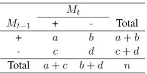
For practical applications we will not know the true population probabilities and we will have to resort to using sample estimates. The SP method uses a stop set of sizenfor deriving its estimates.
Table 2 shows the contingency table counts for the classifications of models Mt and Mt−1 on a
sample of sizen. The population probabilitiesπij
can be estimated by the relative frequenciespijfor i, j∈ {+,−, .}, where:p++ =a/n;p+−=b/n;
p−+=c/n;p−−=d/n;p+.= (a+b)/n;p−.= (c+d)/n;p.+= (a+c)/n; andp.−= (c+d)/n. Letpo =p+++p−−, the observed proportion of agreement and letpe=p+.p.++p−.p.−, the pro-portion of agreement expected by chance if we as-sume thatMtandMt−1make their classifications
independently. Then the Kappa measure of agree-ment K betweenMtandMt−1(see Equation 3) is
estimated by
ˆ
K = po−pe 1−pe
Mt
Mt−1 + - Total
+ a b a+b
- c d c+d
[image:4.595.109.255.60.133.2]Total a+c b+d n
Table 2: Contingency table counts forMt(model
learned at iteration t) andMt−1(model learned at
iteration t-1).
Using the delta method, as described in (Bishop et al., 1975), Fleiss et al. (1969) derived an estima-tor of the large-sample variance ofKˆ. According
to Hale and Fleiss (1993), the estimator simplifies to
V ar( ˆK) = 1 n(1−pe)2×
( X
i∈{+,−}
pii[1−4¯pi(1−K)]ˆ
−( ˆK−pe(1−K))ˆ 2+ (1−K)ˆ 2×
X
i,j∈{+,−}
pij[2(¯pi+ ¯pj)−(pi.+p.j)]2
)
,
(5)
where p¯i = (pi.+p.i)/2. From Equation 5, we
can see that the variance of our estimate of Kappa is inversely proportional to the size of the stop set we use.
Bloodgood and Vijay-Shanker (2009a) used a stop set of size 2000 for each of their datasets. Although this worked well in the results they re-ported, we do not believe that 2000 is a fixed size that will work well for all tasks and datasets where the SP method could be used. Table 3 shows the variances of Kˆ computed using Equation 5
at the points at which SP stopped AL for each of the datasets4from (Bloodgood and Vijay-Shanker, 2009a).
These variances indicate that the size of 2000 was typically sufficient to get tight estimates of Kappa, helping to illuminate the empirical success of the SP method on these datasets. More gener-ally, the SP method can be augmented with a vari-ance check: if the varivari-ance of estimated Kappa at a potential stopping point exceeds some desired
4We note that each of the datasets was set up as a binary
classification task (or multiple binary classification tasks). Further details and descriptions of each of the datasets can be found in (Bloodgood and Vijay-Shanker, 2009a).
threshold, then the stop set size can be increased as needed to reduce the variance.
Looking at Equation 5 again, one can note that whenpeis relatively close to 1, the variance ofKˆ
can be expected to get quite large. In these situ-ations, users of SP should expect to have to use larger stop set sizes and in extreme conditions, SP may not be an advisable method to use.
3.2 Relationship between Kappa agreement and change in performance between models
Heretofore, the published literature contained only informal explanations of why stabilizing predic-tions is expected to work well as a stopping method (along with empirical tests demonstrat-ing successful operation on a handful of tasks and datasets). In the remainder of this section we describe the mathematical foundations for stop-ping methods based on stabilizing predictions. In particular, we will prove that even in the worst possible case, if the Kappa agreement between two subsequently learned models is greater than a threshold T, then it must be the case that the
change in performance between these two models is bounded above by 4(1−T)
T . We then go on to
prove additional Theorems that tighten this bound when assumptions are made about model preci-sion.
Lemma 3.1 Suppose F-measureF and KappaK
are computed from the same contingency table of counts, such as the one given in Table 2. Suppose ad−bc≥0. ThenF ≥K.
Proof By definition, in terms of the contingency table counts,
K = 2ad−2bc
(a+b)(b+d) + (a+c)(c+d) (6)
and
F = 2a
2a+b+c. (7)
RewritingF so that it will have the same
numera-tor asK, we have:
F = F d− bc
a d−bca
!
(8)
= 2a
2a+b+c
d−bc a d−bca
!
(9)
= 2ad−2bc
2ad+bd+cd−2bc−b2c+bc2 a
[image:4.595.82.293.296.426.2]Task-Dataset Variance ofKˆ
NER-DNA (10-fold CV) 0.0000223 NER-cellType (10-fold CV) 0.0000211 NER-protein (10-fold CV) 0.0000074 Reuters (10 Categories) 0.0000298 20 Newsgroups (20 Categories) 0.0000739 WebKB Student (10-fold CV) 0.0000137 WebKB Project (10-fold CV) 0.0000190 WebKB Faculty (10-fold CV) 0.0000115 WebKB Course (10-fold CV) 0.0000179 TC-spamassassin (10-fold CV) 0.0000042 TC-TREC-SPAM (10-fold CV) 0.0000043
[image:5.595.186.412.59.248.2]Average (macro-avg) 0.0000209
Table 3: Estimates of the variance ofKˆ. For each dataset, the estimate of the variance ofKˆ is computed
(using Equation 5) from the contingency table at the point at which SP stopped AL and the average of all the variances (across all folds of CV) is displayed. The last row contains the macro-average of the average variances for all the datasets.
We can see that the expression for F in
Equa-tion 10 has the same numerator as K in Equa-tion 6 but the denominator ofKin Equation 6 is≥
the denominator ofF in Equation 10. Therefore, F ≥K.
Theorem 3.2 LetMtbe the model learned at iter-ationtof active learning andMt−1 be the model learned at iterationt−1. LetKtbe the estimate of Kappa agreement between the classifications of MtandMt−1on the examples in the stop set. Let
˜
Ftbe the F-measure between the classifications of Mtand truth on the stop set. Let F˜t−1 be the F-measure between the classifications ofMt−1 and truth on the stop set. Let∆FtbeF˜t−F˜t−1. Sup-poseT >0. ThenKt> T ⇒ |∆Ft| ≤ 4(1T−T).
Proof Suppose Mt, Mt−1, Kt, F˜t, F˜t−1, ∆Ft,
and T are defined as stated in the statement of
Theorem 3.2. Let Ft be the F-measure between
the classifications ofMt andMt−1 on the
exam-ples in the stop set. Let Table 2 show the con-tingency table counts forMt versusMt−1 on the
examples in the stop set. Then, from their defi-nitions, we haveKt = (a+b)(b+d)+(a+c)(c+d)2(ad−bc) and Ft = 2a+b+c2a . There exist true labels for the
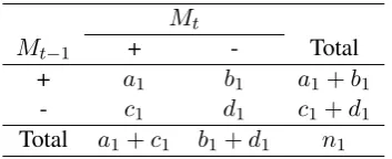
ex-amples in the stop set, which we don’t know since the stop set is unlabeled, but nonetheless must ex-ist. We use the truth on the stop set to split Table 2 into two subtables of counts, one table for all the examples that are truly positive and one table for all the examples that are truly negative. Table 4
Mt
Mt−1 + - Total
+ a1 b1 a1+b1
- c1 d1 c1+d1
[image:5.595.329.506.333.405.2]Total a1+c1 b1+d1 n1
Table 4: Contingency table counts forMt(model
learned at iteration t) versusMt−1 (model learned
at iteration t-1) for only the examples in the stop set that have truth = +1.
Mt
Mt−1 + - Total
+ a−1 b−1 a−1+b−1
- c−1 d−1 c−1+d−1
Total a−1+c−1 b−1+d−1 n−1
Table 5: Contingency table counts forMt(model
learned at iteration t) versusMt−1 (model learned
at iteration t-1) for only the examples in the stop set that have truth = -1.
shows the contingency table forMtversusMt−1
for all of the examples in the stop set that have true labels of +1 and Table 5 shows the contingency ta-ble forMtversusMt−1 for all of the examples in
the stop set that have true labels of -1.
From Tables 2, 4, and 5 one can see that ais
the number of examples in the stop set that both
MtandMt−1 classified as positive. Furthermore,
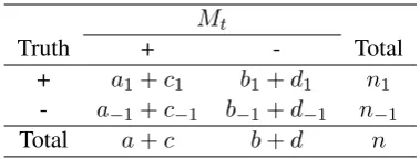
[image:5.595.308.524.484.554.2]pos-Mt
Truth + - Total
+ a1+c1 b1+d1 n1
- a−1+c−1 b−1+d−1 n−1
[image:6.595.86.276.61.133.2]Total a+c b+d n
Table 6: Contingency table counts forMt(model
learned at iteration t) versus truth. (Derived from Tables 4 and 5
Mt−1
Truth + - Total
+ a1+b1 c1+d1 n1
- a−1+b−1 c−1+d−1 n−1
Total a+b c+d n
Table 7: Contingency table counts for Mt−1
(model learned at iteration t-1) versus truth. (De-rived from Tables 4 and 5
itive and a−1 of them truly are negative. Similar
explanations hold for the other counts. Also, from Tables 2, 4, and 5, one can see that the equalities
a= a1+a−1,b = b1+b−1,c =c1+c−1, and d = d1 +d−1 all hold. The contingency tables
forMtversus truth andMt−1versus truth can be
derived from Tables 4 and 5. For convenience, Ta-ble 6 shows the contingency taTa-ble for Mt versus
truth and Table 7 shows the contingency table for
Mt−1 versus truth. Suppose that Kt > T. This
implies, by Lemma 3.15, that F
t > T. This
im-plies that
2a
2a+b+c > T (11)
⇒ 2a >(2a+b+c)T (12)
⇒ 2a(1−T)>(b+c)T (13)
⇒ b+c < 2a(1T−T). (14)
Note that Equations 12 and 14 are justified since
2a+b+c >0andT >0, respectively.
From Table 6 we can see that
˜
Ft= 2(a1+c1)+b1+d1+a2(a1+c1) −1+c−1; from Table 7
we can see thatF˜t
−1 = 2(a1+b1)+c1+d1+a2(a1+b1) −1+b−1.
For notational convenience, let: g = 2(a1 + c1) + b1 + d1 + a−1 + c−1; and h= 2(a1+b1) +c1+d1+a−1+b−1.
5Note that the conditionad−bc ≥ 0of Lemma 3.1 is
met sinceKt > T andT >0implyKt >0, which in turn
impliesad−bc >0.
It follows that
∆Ft=
2(a1+c1)
g −
2(a1+b1)
h (15)
= (2a1+ 2c1)h−(2a1+ 2b1)g
gh (16)
For notational convenience, let: x = 2(a1c1 + a1b−1 +c21 +c1d1 +c1a−1 +c1b−1); andy = 2(a1b1 +a1c−1 +b21+b1d1 +b1a−1 +b1c−1).
Then picking up from Equation 16, it follows that
∆Ft= x−y
gh (17)
= 2[u1+c1u2−b1u3]
gh , (18)
whereu1 =a1c1−a1b1+a1b−1−a1c−1,u2 = c1+d1+a−1+b−1, andu3 =b1+d1+a−1+c−1.
For notational convenience, let: dA = c1−b1
anddB =c−1−b−1. Then it follows that
∆Ft= 2u4
gh, (19)
where:u4=a1(dA−dB) +dA(d1+a−1+b1+ c1) +c1b−1−b1c−1.
Noting thatg=h+dA+dB, we have
∆Ft=
2u4 h(h+dA+dB)
. (20)
Noting that 2u4 = 2[dA(a1 +b1+c1+d1 + a−1+b−1)−dB(a1+b1)]and lettingu5=a1+ b1+c1+d1+a−1+b−1, we have
∆Ft=
2[dAu5−dB(a1+b1)] h(h+dA+dB)
. (21)
Therefore,
|∆Ft| ≤2
dAu5 h(h+dA+dB)
+
h(hdB+(ad1A++b1d)B)
! (22)
Recall thatb+c=b1+b−1+c1+c−1. Then
observe that the following three inequalities hold:
b+c≥dA;b+c≥dB; andh(h+dA+dB)>0.
Therefore,
|∆Ft| ≤ 2(b+c)[2a1+2b1h(h+d+c1+d1+aA+dB) −1+b−1] (23)
= h(h+d2(b+c)h
A+dB) (24)
= h+d2(b+c)
A+dB (25)
≤ T2(2a)(1(h+dA−+dTB)) (26)
= 4(1T−T) h+da
A+dB
[image:6.595.86.277.198.268.2]
Observe thath+dA+dB = 2a1+b1+ 2c1+d1+ a−1+c−1. Therefore, h+dAa+dB ≤1. Therefore,
we have
|∆Ft| ≤
4(1−T)
T . (28)
Note that in deriving Inequality 26, we used the previously derived Inequality 14. Also, the proof of Theorem 3.2 assumes a worst possible case in the sense that all examples where the clas-sifications of Mt and Mt−1 differ are assumed
to have truth values that all serve to maximize one model’s F-measure and minimize the other model’s F-measure so as to maximize |∆Ft| as
much as possible. A resulting limitation is that the bound is loose in many cases. It may be possible to derive tighter bounds, perhaps by easing off to an expected case instead of a worst case and/or by making additional assumptions.6
Taking this possibility up, we now prove tighter bounds when assumptions about the precision of the modelsMtandMt−1 are made. Consider that
in the proof of Theorem 3.2 when transitioning from Equality 27 to Inequality 28, we used the fact that a
h+dA+dB ≤ 1. Note that
a h+dA+dB =
a
2a1+b1+2c1+d1+a−1+c−1, from which one sees that a
h+dA+dB = 1only if all ofa1, b1, c1, d1 andc−1 are all zero. This is a pathological case. In many practically important classes of cases to consider,
a
h+dA+dB will be strictly less than1, and often sub-stantially less than1. The following two Theorems
prove tighter bounds on |∆Ft|than Theorem 3.2
by utilizing this insight.
Theorem 3.3 Suppose Mt, Mt−1, Kt, F˜t, F˜t−1, ∆Ft, andT are defined as stated in the statement of Theorem 3.2. Let the contingency tables be de-fined as they were in the proof of Theorem 3.3. Let MP ositiveConjunction be a model that only clas-sifies an example as positive if both models Mt andMt−1 classify the example as positive. Sup-pose that MP ositiveConjunction has perfect preci-sion on the stop set, or in other words that every single example from the stop set that bothMtand Mt−1classify as positive is truthfully positive (i.e., a−1= 0). ThenKt> T ⇒ |∆Ft| ≤ 2(1T−T).
Proof The proof of Theorem 3.2 holds exactly as it is up until Equality 27. Now, using the additional assumption that a−1 = 0, we have
6If one is planning to undertake this challenge, we would
suggest further consideration of Inequalities 22, 23, 26, and 28 as a possible starting point.
a h+dA+dB ≤
1
2. Therefore, we have
|∆Ft| ≤
2(1−T)
T . (29)
Theorem 3.3 is a special case (in the limit) of a more general Theorem. Before stating and prov-ing the more general Theorem, we prove a Lemma that will be helpful in making the proof of the gen-eral Theorem clearer.
Lemma 3.4 Let f, dA, dB and contingency ta-ble counts be defined as they were in the proof of Theorem 3.2. Suppose a1 = xa−1. Then
a h+dA+dB ≤
x+1 2x+1.
Proof a1 = xa−1 by hypothesis. a = a1 +a−1
by definition of contingency table counts. Hence,
a= (x+ 1)a−1. Therefore,
a
h+dA+dB ≤
(x+1)a−1
2xa−1+a−1 (30)
= (x+1)a−1 (2x+1)a−1 = 2x+1x+1.
The following Theorem generalizes Theo-rem 3.3 to cases when MP ositiveConjunction has
precisionpin(0,1).7
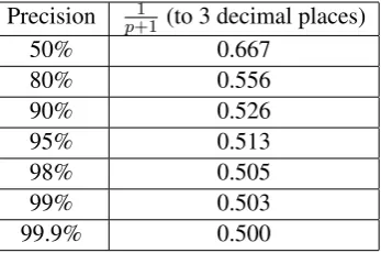
Theorem 3.5 Suppose Mt, Mt−1, Kt, F˜t, F˜t−1, ∆Ft, andT are defined as stated in the statement of Theorem 3.2. Let the contingency tables be de-fined as they were in the proof of Theorem 3.2. Let MP ositiveConjunction be a model that only classi-fies an example as positive if both modelsMtand Mt−1 classify the example as positive. Suppose that MP ositiveConjunction has precision p on the stop set. ThenKt> T ⇒ |∆Ft| ≤ 4(1(p+1)T−T).
Proof The proof of Theorem 3.2 holds exactly as it is up until Equality 27.MP ositiveConjunctionhas
precisionpon the stop set⇒ p = a1+aa1
−1.
Solv-ing fora1 in terms ofa−1 we havea1 = 1−ppa−1.
Therefore, applying Lemma 3.4 withx= 1−pp, we
have a
h+dA+dB ≤ p
1−p+1
2p
1−p+1
. Therefore we have
|∆Ft| ≤ 4
p
1−p+1
2p
1−p+1
!
(1−T)
T (31)
= 4(1(p+1)T−T). (32)
7The case whenp= 0is handled by Theorem 3.2 and the
Precision 1
p+1 (to 3 decimal places)
50% 0.667
80% 0.556
90% 0.526
95% 0.513
98% 0.505
99% 0.503
[image:8.595.96.270.62.177.2]99.9% 0.500
Table 8: Values of the scaling factor from Theo-rem 3.5 for different precision values.
The scaling factor 1
p+1 in Theorem 3.5 shows
how the precision of the conjunctive model affects the bound. Theorem 3.2 had the scaling factor im-plicitly set to 1 in order to handle the pathologi-cal case where the positive conjunctive model has precision = 0. In Theorem 3.3, where the positive conjunctive model has precision = 1 on the exam-ples in the stop set, the scaling factor is set to 1/2. Theorem 3.5 generalizes the scaling factor so that it is a function of the precision of the positive con-junctive model. For convenience, Table 8 shows the scaling factor values for a few different preci-sion values.
The bounds in Theorems 3.2, 3.3, and 3.5 all bound the difference in performance on the stop set of two consecutively learned models Mt and Mt−1. An issue to consider is how connected the
difference in performance on the stop set is to the difference in performance on a stream of applica-tion examples generated according to the popula-tion probabilities. Taking up this issue, consider that the proof of Theorems 3.2, 3.3, and 3.5 would hold as it is if we had used sample proportions in-stead of sample counts (this can be seen by simply dividing every count byn, the size of the stop set).
Since the stop set is unbiased (selected at random from the population), asnapproaches infinity, the
sample proportions will approach the population probabilities and the difference between the dif-ference in performance betweenMtandMt−1on
the stop set and on a stream of application exam-ples generated according to the population proba-bilities will approach zero.
4 Conclusions
To date, the work on stopping criteria has been dominated by heuristics based on intuitions and experimental success on a small handful of tasks
and datasets. But the methods are not widely usable in practice yet because our community’s understanding of the stopping methods remains too inexact. Pushing forward on understanding the mechanics of stopping at a more exact level is therefore crucial for achieving the design of widely usable effective stopping criteria.
This paper presented the first theoretical anal-ysis of stopping based on stabilizing predictions. The analysis revealed three elements that are cen-tral to the SP method’s success: (1) the sample es-timates of Kappa have low variance; (2) Kappa has tight connections with differences in F-measure; and (3) since the stop set doesn’t have to be la-beled, it can be arbitrarily large, helping to guar-antee that the results transfer to previously unseen streams of examples at test/application time.
We presented proofs of relationships between the level of Kappa agreement and the difference in performance between consecutive models. Specif-ically, if the Kappa agreement between two mod-els is at least T, then the difference in F-measure performance between those models is bounded above by 4(1−T)
T . If precision of the positive
con-junction of the models is assumed to bep, then the
bound can be tightened to 4(1−T) (p+1)T.
The setup and methodology of the proofs can serve as a launching pad for many further inves-tigations, including: analyses of stopping; works that consider switching between different active learning strategies and operating regions; and works that consider stopping co-training, and es-pecially agreement-based co-training. Finally, the relationships that have been exposed between the Kappa statistic and F-measure may be of broader use in works that consider inter-annotator agree-ment and its interplay with system evaluation, a topic that has been of long-standing interest.
References
Shlomo Argamon-Engelson and Ido Dagan. 1999. Committee-based sample selection for probabilis-tic classifiers. Journal of Artificial Intelligence Re-search (JAIR), 11:335–360.
Ron Artstein and Massimo Poesio. 2008. Inter-coder
agreement for computational linguistics.
Computa-tional Linguistics, 34(4):555–596.
Jason Baldridge and Miles Osborne. 2008.
Yoram Baram, Ran El-Yaniv, and Kobi Luz. 2004. On-line choice of active learning algorithms. Journal of Machine Learning Research, 5:255–291, March. Yvonne M. Bishop, Stephen E. Fienberg, and Paul W.
Holland. 1975. Discrete Multivariate Analysis:
Theory and Practice. MIT Press, Cambridge, MA. Michael Bloodgood and Chris Callison-Burch. 2010.
Bucking the trend: Large-scale cost-focused active learning for statistical machine translation. In Pro-ceedings of the 48th Annual Meeting of the Associa-tion for ComputaAssocia-tional Linguistics, pages 854–864, Uppsala, Sweden, July. Association for Computa-tional Linguistics.
Michael Bloodgood and K Vijay-Shanker. 2009a. A method for stopping active learning based on stabi-lizing predictions and the need for user-adjustable
stopping. InProceedings of the Thirteenth
Confer-ence on Computational Natural Language Learning (CoNLL-2009), pages 39–47, Boulder, Colorado, June. Association for Computational Linguistics. Michael Bloodgood and K Vijay-Shanker. 2009b.
Tak-ing into account the differences between actively and passively acquired data: The case of active learning with support vector machines for
imbal-anced datasets. In Proceedings of Human
Lan-guage Technologies: The 2009 Annual Conference of the North American Chapter of the Associa-tion for ComputaAssocia-tional Linguistics, pages 137–140, Boulder, Colorado, June. Association for Computa-tional Linguistics.
Michael Bloodgood. 2009. Active learning with
sup-port vector machines for imbalanced datasets and a method for stopping active learning based on sta-bilizing predictions. Ph.D. thesis, University of Delaware, Newark, DE, USA.
Avrim Blum and Tom Mitchell. 1998. Combining la-beled and unlala-beled data with co-training. InCOLT’ 98: Proceedings of the eleventh annual conference on Computational learning theory, pages 92–100, New York, NY, USA. ACM.
J. Carletta. 1996. Assessing agreement on classifica-tion tasks: The kappa statistic. Computational lin-guistics, 22(2):249–254.
Stephen Clark, James Curran, and Miles Osborne. 2003. Bootstrapping pos-taggers using unlabelled data. In Walter Daelemans and Miles Osborne,
editors, Proceedings of the Seventh Conference on
Natural Language Learning at HLT-NAACL 2003, pages 49–55.
J. Cohen. 1960. A coefficient of agreement for
nom-inal scales. Educational and Psychological
Mea-surement, 20:37–46.
David A. Cohn, Zoubin Ghahramani, and Michael I. Jordan. 1996. Active learning with statistical mod-els. Journal of Artificial Intelligence Research, 4:129–145.
Meryem Pinar D¨onmez, Jaime G. Carbonell, and
Paul N. Bennett. 2007. Dual strategy active
learning. In Joost N. Kok, Jacek Koronacki,
Ramon L´opez de M´antaras, Stan Matwin, Dunja
Mladenic, and Andrzej Skowron, editors, Machine
Learning: ECML 2007, 18th European Conference on Machine Learning, Warsaw, Poland, September 17-21, 2007, Proceedings, volume 4701 of Lec-ture Notes in Computer Science, pages 116–127. Springer.
Seyda Ertekin, Jian Huang, L´eon Bottou, and C. Lee Giles. 2007a. Learning on the border: active learn-ing in imbalanced data classification. In M´ario J. Silva, Alberto H. F. Laender, Ricardo A. Baeza-Yates, Deborah L. McGuinness, Bjørn Olstad, Øys-tein Haug Olsen, and Andr´e O. Falc˜ao, editors, Pro-ceedings of the Sixteenth ACM Conference on Infor-mation and Knowledge Management, CIKM 2007, Lisbon, Portugal, November 6-10, 2007, pages 127– 136. ACM.
Seyda Ertekin, Jian Huang, and C. Lee Giles. 2007b. Active learning for class imbalance problem. In Wessel Kraaij, Arjen P. de Vries, Charles L. A. Clarke, Norbert Fuhr, and Noriko Kando, editors,
SIGIR 2007: Proceedings of the 30th Annual Inter-national ACM SIGIR Conference on Research and Development in Information Retrieval, Amsterdam, The Netherlands, July 23-27, 2007, pages 823–824. ACM.
Joseph L. Fleiss, Jacob Cohen, and B. S. Everitt. 1969. Large sample standard errors of kappa and weighted kappa. Psychological Bulletin, 72(5):323 – 327. Yoav Freund, H. Sebastian Seung, Eli Shamir, and
Naf-tali Tishby. 1997. Selective sampling using the
query by committee algorithm. Machine Learning,
28:133–168.
Masood Ghayoomi. 2010. Using variance as a stop-ping criterion for active learning of frame
assign-ment. In Proceedings of the NAACL HLT 2010
Workshop on Active Learning for Natural Language Processing, pages 1–9, Los Angeles, California, June. Association for Computational Linguistics. Ben Hachey, Beatrice Alex, and Markus Becker. 2005.
Investigating the effects of selective sampling on the annotation task. InProceedings of the Ninth Confer-ence on Computational Natural Language Learning (CoNLL-2005), pages 144–151, Ann Arbor, Michi-gan, June. Association for Computational Linguis-tics.
Robbie Haertel, Eric Ringger, Kevin Seppi, James Car-roll, and Peter McClanahan. 2008. Assessing the costs of sampling methods in active learning for
an-notation. InProceedings of ACL-08: HLT, Short
Pa-pers, pages 65–68, Columbus, Ohio, June.
Associa-tion for ComputaAssocia-tional Linguistics.
Gholamreza Haffari and Anoop Sarkar. 2009. Active learning for multilingual statistical machine
the 47th Annual Meeting of the ACL and the 4th In-ternational Joint Conference on Natural Language Processing of the AFNLP, pages 181–189, Suntec, Singapore, August. Association for Computational Linguistics.
Cecilia A. Hale and Joseph L. Fleiss. 1993. Interval es-timation under two study designs for kappa with bi-nary classifications. Biometrics, 49(2):pp. 523–534. Rebecca Hwa. 2000. Sample selection for statistical grammar induction. In Hinrich Sch¨utze and Keh-Yih Su, editors,Proceedings of the 2000 Joint SIG-DAT Conference on Empirical Methods in Natural Language Processing, pages 45–53. Association for Computational Linguistics, Somerset, New Jersey. Florian Laws and Hinrich Sch¨utze. 2008. Stopping
cri-teria for active learning of named entity recognition. InProceedings of the 22nd International Conference on Computational Linguistics (Coling 2008), pages 465–472, Manchester, UK, August. Coling 2008 Or-ganizing Committee.
David D. Lewis and William A. Gale. 1994. A se-quential algorithm for training text classifiers. In SI-GIR ’94: Proceedings of the 17th annual interna-tional ACM SIGIR conference on Research and de-velopment in information retrieval, pages 3–12, New York, NY, USA. Springer-Verlag New York, Inc. D. Roth and K. Small. 2008. Active learning for
pipeline models. In Proceedings of the National
Conference on Artificial Intelligence (AAAI), pages 683–688.
Nicholas Roy and Andrew McCallum. 2001. Toward optimal active learning through sampling estimation of error reduction. InIn Proceedings of the 18th In-ternational Conference on Machine Learning, pages 441–448. Morgan Kaufmann.
Manabu Sassano. 2002. An empirical study of active learning with support vector machines for japanese
word segmentation. InACL ’02: Proceedings of the
40th Annual Meeting on Association for Computa-tional Linguistics, pages 505–512, Morristown, NJ, USA. Association for Computational Linguistics. Greg Schohn and David Cohn. 2000. Less is more:
Active learning with support vector machines. In
Proc. 17th International Conf. on Machine
Learn-ing, pages 839–846. Morgan Kaufmann, San
Fran-cisco, CA.
Burr Settles and Mark Craven. 2008. An analysis of active learning strategies for sequence labeling
tasks. In Proceedings of the 2008 Conference on
Empirical Methods in Natural Language
Process-ing, pages 1070–1079, Honolulu, Hawaii, October.
Association for Computational Linguistics.
H. S. Seung, M. Opper, and H. Sompolinsky. 1992.
Query by committee. InCOLT ’92: Proceedings of
the fifth annual workshop on Computational learn-ing theory, pages 287–294, New York, NY, USA. ACM.
Dan Shen, Jie Zhang, Jian Su, Guodong Zhou, and Chew-Lim Tan. 2004. Multi-criteria-based ac-tive learning for named entity recognition. In Pro-ceedings of the 42nd Meeting of the Association for Computational Linguistics (ACL’04), Main Volume, pages 589–596, Barcelona, Spain, July.
Cynthia A. Thompson, Mary Elaine Califf, and Ray-mond J. Mooney. 1999. Active learning for natural
language parsing and information extraction. InIn
Proceedings of the 16th International Conference on Machine Learning, pages 406–414. Morgan Kauf-mann, San Francisco, CA.
Katrin Tomanek, Joachim Wermter, and Udo Hahn.
2007. An approach to text corpus construction
which cuts annotation costs and maintains
reusabil-ity of annotated data. In Proceedings of the 2007
Joint Conference on Empirical Methods in Natural Language Processing and Computational Natural Language Learning (EMNLP-CoNLL), pages 486– 495.
Andreas Vlachos. 2008. A stopping criterion for
active learning. Computer Speech and Language,
22(3):295–312.
Jingbo Zhu and Eduard Hovy. 2007. Active learn-ing for word sense disambiguation with methods for
addressing the class imbalance problem. In
Pro-ceedings of the 2007 Joint Conference on Empirical Methods in Natural Language Processing and Com-putational Natural Language Learning (EMNLP-CoNLL), pages 783–790.
Jingbo Zhu, Huizhen Wang, and Eduard Hovy. 2008a. Learning a stopping criterion for active learning for word sense disambiguation and text classification. InIJCNLP.