The Language of Place: Semantic Value from Geospatial Context

The Language of Place: Semantic Value from Geospatial Context

Anne Cocos and Chris Callison-Burch

University of Pennsylvania

[email protected] [email protected]

Abstract

There is a relationship between what we say and where we say it. Word embed-dings are usually trained assuming that semantically-similar words occur within the sametextual contexts. We investigate the extent to which semantically-similar words occur within the same geospatial

contexts. We enrich a corpus of ge-olocated Twitter posts with physical data derived from Google Places and Open-StreetMap, and train word embeddings us-ing the resultus-ing geospatial contexts. In-trinsic evaluation of the resulting vectors shows that geographic context alone does provide useful information about semantic relatedness.

1 Introduction

Words follow geographic patterns of use. At times the relationship is obvious; we would expect to hear conversations about actors in and around a movie theater. Other times the connection be-tween location and topic is less clear; people are more likely to tweet about something they love

from a bar than from home, but vice versa for something they hate.1 _{Distributional semantics}

is based on the theory that semantically similar words occur within the sametextualcontexts. We question the extent to which similar words occur within the samegeospatialcontexts.

Previous work validates the relationship be-tween the content of text and its physical origin. Geographically-grounded models of language en-able toponym resolution (DeLozier et al., 2015), 1_{Under our GEO30 word embeddings, the word love} is closer to the context GooglePlaces:bar than to high-way:residential. The relationship is inverted for the word hate.

document origin prediction, (Wing and Baldridge, 2011; Hong et al., 2012; Han et al., 2012b; Han et al., 2013; Han et al., 2014) and tracking re-gional variation in word use (Eisenstein et al., 2010; Eisenstein et al., 2014; Bamman et al., 2014; Huang et al., 2016). Our work differs from earlier models; rather than modeling lan-guage with respect to an absolute, physical loca-tion (like a geographic bounding box), we model language with respect to attributes describing a type of location (like amenity:movie theater or

landuse:residential). This allows us to model the impact of geospatial context independently of lan-guage and region.

We enrich a corpus of geolocated tweets with geospatial information describing the physical en-vironment where they were posted. We use the geospatial contexts to train geo-word embed-dings with theskip-gram with negative sampling

(SKIPGRAM) model (Mikolov et al., 2013) as

adapted to support arbitrary contexts (Levy and Goldberg, 2014). We then demonstrate the seman-tic value of geospatial context in two ways. First, using intrinsic methods of evaluation, we show that the resulting geo-word embeddings them-selves encode information about semantic related-ness. Second, we present initial results suggest-ing that because the embeddsuggest-ings are trained with language-agnostic features, they give a potentially useful signal about bilingual translation pairs.

2 Geo-enriching Tweets

We collected 6.2 million geolocated English tweets in 20 metro areas from Jan-Mar 2016.2 _The

2_{The metro areas, chosen based on high volume of} ge-olocated tweets collected during an initial trial period, were Atlanta, Bandung, Bogota, Buenos Aires, Chicago, Dal-las, Washington DC, Houston, Istanbul, Jakarta, Los An-geles, London, Madrid, Mexico City, Miami, New York City, Philadelphia, San Francisco Bay Area, Singapore, and Toronto. We used only tweets explicitly tagged with

tokens in these tweets were normalized by con-verting to lowercase, replacing @-mentions, num-bers, and URLs with special symbols, and apply-ing the lexical normalization dictionary of Han et al. (2012a).

To enrich our collected tweets with geospa-tial features, we used publicly-available geospageospa-tial data from OpenStreetMap and the Google Places API. OpenStreetMap (OSM) is a crowdsourced mapping initiative. Users provide surveyed data such as administrative boundaries, land use, and road networks in their local area. In addition to ge-ographic coordinates, each shape in the data set in-cludes tags describing its type and attributes, such asshop:convenienceandbuilding:retailfor a con-venience store. We downloaded metro extracts for our 20 cities in shapefile format. To maximize coverage, we supplemented the OSM data with Google Places data from its web API, consisting of places tagged with one or more types (i.e. aquar-ium,ATM, etc).

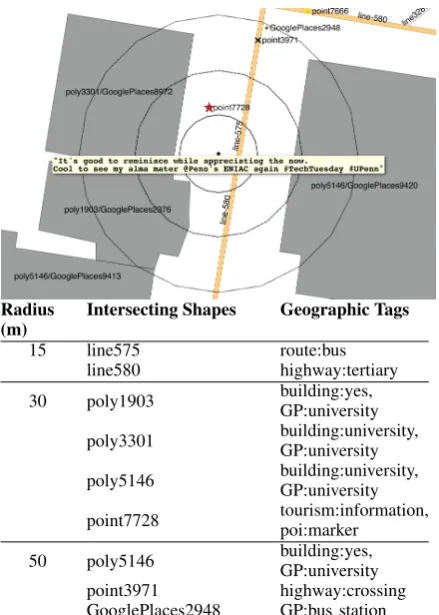
We enrich each geolocated tweet by finding the coordinates and tags for all OSM shapes and Google Places located within 50m of the tweet’s coordinates. The enumerated tags become geo-graphic contexts for training word embeddings. Figure 1 gives an example of geospatial data col-lected for a single tweet.

3 Geo-Word Embeddings

SKIPGRAM learns latent fixed-length vector

rep-resentationsvw andvcfor each word and context in a corpus such that vw · vc is highest for fre-quently observed word-context pairs. Typically a word’s context is modeled as a fixed-length win-dow of words surrounding it. Levy and Gold-berg (2014) generalized SKIPGRAMto accept

ar-bitrary contexts as input. We use their software (word2vecf) to train word embeddings using geospatial contexts.

word2vecf takes a list of (word, context) pairs as input. We train 300-dimensional geo-word embeddings denoted GEOD– whereDindicates a

radius – as follows. For each length-n tweet, we find all shapes within Dmeters of its origin and enumerate the length-m list of the shapes’ geo-graphic tags. The tweet in Figure 1, for example, hasm= 10tags as context when training GEO30

embeddings. Under our model, each token in the tweet shares the same contexts. Thus the input

graphic coordinates.

Radius

(m) Intersecting Shapes Geographic Tags

15 line575 route:bus

line580 highway:tertiary 30 poly1903 building:yes,_{GP:university}

poly3301 building:university,_{GP:university} poly5146 building:university,_{GP:university} point7728 tourism:information,_poi:marker 50 poly5146 building:yes,_{GP:university}

point3971 highway:crossing GooglePlaces2948 GP:bus station

Figure 1: Geoenriching an example tweet with ge-ographic contexts at increasing radii D (meters). For each D ∈ {15,30,50}, geographic contexts include all tags belonging to shapes withinD me-ters of the origin. In this example there are 10 tags for the tweet atD = 30m. GPdenotes tags ob-tained via Google Places; others are from Open-StreetMap.

toword2vecf for training GEO30 embeddings

produced by the example tweet is anm×nlist of (word, context) pairs:

(it’s, route:bus), (good, route:bus), ...

(#TechTuesday, poi:marker), (#UPenn, poi:marker)

The mean number of tags (m) per tweet under each threshold is 12.3 (GEO15), 21.9 (GEO30),

and 38.6 (GEO50). The mean number of tokens

(n) per tweet is 15.7.

4 Intrinsic Evaluation

calcu-late Spearman’s rank correlation between numer-ical human judgements of semantic similarity or relatedness for a large set of word pairs, and the cosine similarity between the same word pairs un-der the geo-word embedding models.

To understand the impact of geographic con-texts on the embedding model, we compare GEO15, GEO30, and GEO50 geo-word

embed-dings to the following baselines:

TEXT5: Using our corpus of geolocated tweets, we train word embeddings withword2vecf us-ing traditional linear bag-of-words contexts with window width 5.

GEO30+TEXT5: We also evaluate the impact of combining textual and geospatial contexts. We train a model over the geolocated tweets corpus using both the geospatial contexts from GEO30

and the textual contexts from TEXT5.

RAND30: Because our GEOD models assign

the same geospatial contexts to every token in a tweet, we need to rule out the possibility that GEOD models are simply capturing relatedness

between words that frequently appear in the same tweets, like movie and theater. We implement a random baseline model that captures similar-ities arising from tweet co-location alone. For each tweet, we enumerate the geospatial tags (i.e. contexts) for shapes within 30m of the tweet ori-gin. Then, before feeding the m × n list of (word, context) pairs to word2vecf for train-ing, we randomly map each tag type to a dif-ferent tag type within the context vocabulary. For example, route:bus could be mapped to amenity:bankfor input to the model. We redo the random tag mapping for each tweet. In this way, vectors for words that always appear together within tweets are trained on the same set of associ-ated contexts. But the randomly mapped contexts do not model the geographic distribution of words.

4.1 Intrinsic Evaluation Results

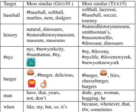
Qualitatively, we find that strongly locational words, like#nyc, and words frequently associated with a type of place, likeburgerandbaseball, tend to have the most semantically and topically simi-lar neighbors (Table 2) . Function words and oth-ers with geographically independent use (i.e.man) have less semantically-similar neighbors.

We can also qualitatively examine the ge-ographic context embeddings vc output by word2vecf. Recall that the SKIPGRAM

objec-Target Most similar (GEO30 ) Most similar (TEXT5)

baseball #baseball, softball,_{marlins, nem, dodgers} softball, lacrosse,#baseball, soccer, tourney

history natural, dinosaurs,#naturalhistorymuseum, museum, museums

#naturalhistorymuseum, smithsonian’s, #museumselfie, #dinosaur, dinosaurs

#nyc

nyc, #newyorkcity,

#manhattan, #ny, #ny, #iloveny,_{#nyclife, #ilovenewyork,} #newyorknewyork

burger , #burger, delicious, ,

#burger, , fries, cheeseburger, burgers

man have, that, years,_{not, don’t} dude, guy, woman,_{hugging, he}

when like, my, but, so, it’s because, whenever, that,_{tfw, sometimes}

Table 2: Most similar words based on cosine sim-ilarity of embeddings trained using geographic contexts within a radius of 30m (GEO30) and

tex-tual contexts with a window of 5 words (TEXT5).

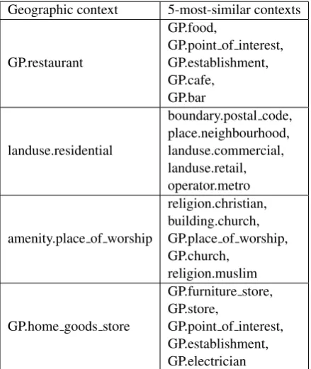
tive function pushes the vectors for frequently co-occurring vc and vw close to one another in a shared vector space. Thus we can find the words (Table 4) and other contexts (Table 3) most closely associated with each geographic context on the ba-sis of cosine similarity. We find qualitatively that the word-context and context-context associations make intuitive sense.

In our intrinsic evaluation (Table 1), geo-word embeddings outperformed the random baseline in six of seven benchmarks. These results are sig-nificant (p < .01) based on the Minimum Re-quired Difference for Significance test of Rastogi et al. (2015). This indicates that geospatial in-formationdoesprovide some useful semantic in-formation. However, the GEODembeddings

un-derperformed the TEXT5 embeddings in all cases.

And although the combined GEO30+TEXT5

em-beddings outperformed the TEXT5 embeddings

Data Set Data Type Rand30 Geo15 Geo30 Geo50 Geo30+Text5 Text5 Ref

MEN rel 0.1372 _{0.319 0.337 0.298 0.528}1 _{0.514 (Bruni et al., 2012)} MTURK-771 rel 0.0762 _{0.224 0.225 0.206 0.357 0.364 (Halawi and Dror, 2012)} WS353-R rel 0.0952 _{0.312 0.334 0.244 0.396 0.382 (Agirre et al., 2009)} WS353-S sim 0.0522 _{0.314 0.275 0.249 0.525 0.555 (Agirre et al., 2009)} RW sim 0.0122 _{0.176 0.167 0.167 0.323 0.362}1 _{(Luong et al., 2013)} SCWS sim 0.3162 _{0.392 0.383 0.385 0.470 0.499}1 _{(Huang et al., 2012)} SimLex sim 0.081 0.069 0.068 0.052 0.100 0.1921 _{(Hill et al., 2015)} 1_{Indicates a significant difference between TEXT5 and GEO30+TEXT5 results (p <0.05, (Rastogi et al., 2015))}

2_{Indicates RAND30 results are significantly lower than any GEOor WORDembedding results (p <0.01, (Rastogi et al., 2015))} Table 1: We calculate the Spearman correlation between pairwise human semantic similarity (sim) and relatedness (rel) judgements, and cosine similarity of the associated word embeddings, over 7 benchmark datasets.

Geographic context 5-most-similar contexts

GP.restaurant

GP.food,

GP.point of interest, GP.establishment, GP.cafe,

GP.bar

landuse.residential

boundary.postal code, place.neighbourhood, landuse.commercial, landuse.retail, operator.metro

amenity.place of worship

religion.christian, building.church, GP.place of worship, GP.church,

religion.muslim

GP.home goods store

GP.furniture store, GP.store,

GP.point of interest, GP.establishment, GP.electrician

Table 3: Most similar contexts, based on cosine similarity of the associated GEO30 context

vec-tors.

below the current state-of-the-art; this is to be ex-pected given the relatively small size of our train-ing corpus (approx. 400M tokens).

5 Translation Prediction

Our intrinsic evaluation established that geospa-tial context provides semantic information about words, but it is weaker than information provided by textual context. So a natural question to ask is whether geospatial context can be useful in any setting. One potential strength of word embed-dings trained using geospatial contexts is that the features are language-independent. Thus we

in-Geospatial context Most similar words (GEO30)

GP.aquarium , , ,

#aquarium, #jellyfish natural.peak #hike, overlook, #hiking,_{coit, mulholland}

amenity.museum history, #dinosaur,#naturalhistorymuseum, american, natural GP.bowling alley , saray, bowling,

idarts, #bowling religion.muslim camii, masjid, sultan,_{mosque, ahmed}

man made.bridge

#bridge, #manhattanbridge, #brooklynbridge, #eastriver,

Table 4: Most similar words for target contexts, based on cosine similarity of their associated GEO30 word and context vectors.

fer that training geo-word embeddings jointly over two languages might yield translation pairs that are close to one another in vector space. This type of model could be applicable in a low-resource language setting where large parallel texts are un-available but geolocated text is. To test this hy-pothesis, we collect an additional 236k geolocated Turkish tweets and re-train GEO30, TEXT5, and

GEO30+TEXT5 vectors on the larger set.

Turk-ish word in the dataset we also select a random English word and add this pair as a negative ex-ample. Our resulting data set has 1056 word pairs, 50% of which are correct translations. We split this into 80% train and 20% test examples.

We construct a logistic regression model, where the input for each word pair is the difference be-tween its Turkish and English word vectors,vf − ve. We evaluate the results using precision, recall, and F-score of positive translation predictions.

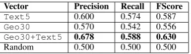
Table 5 gives our results, which we compare to a model that makes a random guess for each word pair. Combining geographic and textual contexts to train embeddings leads to better translation per-formance than using textual or geospatial contexts in isolation. In particular, with a seed dictionary of just 528 Turkish words and monolingual text of just 236k tweets, our supervised method is able to predict correct translation pairs with 67.8% preci-sion. While the not signficant under McNemar’s test (p=0.07), they are suggestive that geospatial contextual information may provide a useful sig-nal for bilingual lexicon induction when used in combination with other methods, as in Irvine and Callison-Burch (2013).

Vector Precision Recall FScore

Text5 0.600 0.574 0.587

Geo30 0.570 0.542 0.556

Geo30+Text5 0.678 0.588 0.630

Random 0.500 0.500 0.500

Table 5: We make a binary translation prediction for Turkish-English word pairs using their embed-dings in a simple logistic regression model.

6 Conclusion

Typically word embeddings are generated using thetextsurrounding a word as context from which to derive semantic information. We explored what happens when we use thegeospatialcontext – in-formation about the physical location where text originates – instead. Intrinsic evaluation of word embeddings trained over a set of geolocated Twit-ter data, using geospatial information derived from OpenStreetMap and the Google Places API as context, indicated that the geospatial context does encode information about semantic relatedness.

We also suggested an extrinsic evaluation method for geo-word embeddings: predicting translation pairs without bilingual parallel cor-pora. Our experiments suggested that while

geospatial context is not as semantically-rich as textual context, it does provide useful semantic re-latedness information that may be complementary as part of a multimodal model. As future work, another extrinsic evaluation task that may be ap-propriate forgeo-wordembeddings is geolocation prediction.

Acknowledgments

We would like to thank our reviewers for their thoughtful suggestions. We are also grateful to the National Physical Science Consortium for par-tially funding this work.

References

Eneko Agirre, Enrique Alfonseca, Keith Hall, Jana Kravalova, Marius Pasca, and Aitor Soroa. 2009. A study on similarity and relatedness using distribu-tional and wordnet-based approaches. In Proceed-ings of Human Language Technologies: The 2009 Annual Conference of the North American Chap-ter of the Association for Computational Linguistics, pages 19–27. Association for Computational Lin-guistics.

David Bamman, Chris Dyer, and Noah A. Smith. 2014. Distributed representations of geographically situ-ated language. In Proceedings of the 52nd Annual Meeting of the Association for Computational Lin-guistics (Volume 2: Short Papers), pages 828–834. Association for Computational Linguistics.

Elia Bruni, Gemma Boleda, Marco Baroni, and Khanh Nam Tran. 2012. Distributional semantics in technicolor. In Proceedings of the 50th Annual Meeting of the Association for Computational Lin-guistics (Volume 1: Long Papers), pages 136–145. Association for Computational Linguistics.

Grant DeLozier, Jason Baldridge, and Loretta Lon-don. 2015. Gazetteer-independent toponym resolu-tion using geographic word profiles. InAAAI, pages 2382–2388.

Jacob Eisenstein, Brendan O’Connor, Noah A. Smith, and Eric P. Xing. 2010. A latent variable model for geographic lexical variation. InProceedings of the 2010 Conference on Empirical Methods in Nat-ural Language Processing, pages 1277–1287. Asso-ciation for Computational Linguistics.

Jacob Eisenstein, Brendan O’Connor, Noah A. Smith, and Eric P. Xing. 2014. Diffusion of lexical change in social media. PloS one, 9(11):e113114.

Bo Han, Paul Cook, and Timothy Baldwin. 2012a. Automatically constructing a normalisation dictio-nary for microblogs. In Proceedings of the 2012 Joint Conference on Empirical Methods in ral Language Processing and Computational Natu-ral Language Learning, pages 421–432. Association for Computational Linguistics.

Bo Han, Paul Cook, and Timothy Baldwin. 2012b. Ge-olocation prediction in social media data by finding location indicative words. InProceedings of COL-ING 2012, pages 1045–1062. The COLING 2012 Organizing Committee.

Bo Han, Paul Cook, and Timothy Baldwin. 2013. A stacking-based approach to twitter user geolocation prediction. InProceedings of the 51st Annual Meet-ing of the Association for Computational LMeet-inguis- Linguis-tics: System Demonstrations, pages 7–12. Associa-tion for ComputaAssocia-tional Linguistics.

Bo Han, Paul Cook, and Timothy Baldwin. 2014. Text-based twitter user geolocation prediction. Journal of Artificial Intelligence Research, 49:451– 500.

Felix Hill, Roi Reichart, and Anna Korhonen. 2015. Simlex-999: Evaluating semantic models with (gen-uine) similarity estimation. Computational Linguis-tics, 41(4):665–695.

Liangjie Hong, Amr Ahmed, Siva Gurumurthy, Alexander J. Smola, and Kostas Tsioutsiouliklis. 2012. Discovering geographical topics in the twit-ter stream. In Proceedings of the 21st interna-tional conference on World Wide Web, pages 769– 778. ACM.

Eric Huang, Richard Socher, Christopher Manning, and Andrew Ng. 2012. Improving word represen-tations via global context and multiple word proto-types. InProceedings of the 50th Annual Meeting of the Association for Computational Linguistics (Vol-ume 1: Long Papers), pages 873–882. Association for Computational Linguistics.

Yuan Huang, Diansheng Guo, Alice Kasakoff, and Jack Grieve. 2016. Understanding us regional linguistic variation with twitter data analysis. Computers, En-vironment and Urban Systems, 59:244–255. Ann Irvine and Chris Callison-Burch. 2013.

Su-pervised bilingual lexicon induction with multiple monolingual signals. In Proceedings of the 2013 Conference of the North American Chapter of the Association for Computational Linguistics: Human Language Technologies, pages 518–523. Associa-tion for ComputaAssocia-tional Linguistics.

Omer Levy and Yoav Goldberg. 2014. Dependency-based word embeddings. InProceedings of the 52nd Annual Meeting of the Association for Computa-tional Linguistics (Volume 2: Short Papers), pages 302–308. Association for Computational Linguis-tics.

Thang Luong, Richard Socher, and Christopher Man-ning, 2013. Proceedings of the Seventeenth Confer-ence on Computational Natural Language Learning, chapter Better Word Representations with Recursive Neural Networks for Morphology, pages 104–113. Association for Computational Linguistics.

Tomas Mikolov, Ilya Sutskever, Kai Chen, Greg S. Cor-rado, and Jeff Dean. 2013. Distributed representa-tions of words and phrases and their compositional-ity. InAdvances in Neural Information Processing Systems, pages 3111–3119.

Ellie Pavlick, Matt Post, Ann Irvine, Dmitry Kachaev, and Chris Callison-Burch. 2014. The language de-mographics of amazon mechanical turk. Transac-tions of the Association of Computational Linguis-tics, 2:79–92.

Pushpendre Rastogi, Benjamin Van Durme, and Ra-man Arora. 2015. Multiview lsa: Representation learning via generalized cca. InProceedings of the 2015 Conference of the North American Chapter of the Association for Computational Linguistics: Hu-man Language Technologies, pages 556–566. Asso-ciation for Computational Linguistics.