Towards Quantum Language Models

Towards Quantum Language Models

Ivano Basile

Scuola Normale Superiore, Pisa, Italy

[email protected]

Fabio Tamburini

FICLIT - University of Bologna, Italy

[email protected]

Abstract

This paper presents a new approach for building Language Models using the Quantum Probability Theory, a Quantum Language Model (QLM). It mainly shows that relying on this probability calculus it is possible to build stochastic models able to benefit from quantum correlations due to interference and entanglement. We ex-tensively tested our approach showing its superior performances, both in terms of model perplexity and inserting it into an automatic speech recognition evaluation setting, when compared with state-of-the-art language modelling techniques.

1 Introduction

Quantum Mechanics Theory (QMT) is one of the most successful theories in modern science. De-spite its effectiveness in the physics realm, the at-tempts to apply it in other domains remain quite limited, excluding, of course, the large quantity of studies regarding Quantum Information Process-ing on quantum computers.

Only in recent years some scholars tried to em-body principles derived from QMT into their spe-cific fields, for example, by the Information Re-trieval community (Zuccon et al., 2009; Melucci and van Rijsbergen,2011;Gonz´alez and Caicedo, 2011;Melucci, 2015) and in the domain of cog-nitive sciences and decision making (Khrennikov, 2010; Busemeyer and Bruza, 2012; Aerts et al., 2013). In the machine learning field (Arjovsky et al.,2016;Wisdom et al.,2016;Jing et al.,2017) have used unitary evolution matrices for building deep neural networks obtaining interesting results, but we have to observe that their works do not ad-here to QMT and use unitary evolution operators in a way not allowed by QMT. In recent years, also

the Natural Language Processing (NLP) commu-nity started to look at QMT with interest and some studies using it have already been presented (Bla-coe et al.,2013;Liu et al.,2013;Tamburini,2014; Kartsaklis et al.,2016).

Language models (LM) are basic tools in NLP used in various applications, such as Automatic Speech Recognition (ASR), machine translation, part-of-speech tagging, etc., and were traditionally modeled by using N-grams and various smoothing techniques. Among the dozen of tools for comput-ing N-gram LM, we will refer to CMU-SLM (with Good-Turing smoothing) (Clarkson and Rosen-feld,1997) and IRSTLM (with Linear Witten-Bell smoothing) (Federico et al.,2008); the latter is the tool used in Kaldi (Povey et al.,2011b), one of the most powerful and used open-source ASR pack-age that we will use for some of the experiments presented in the following sections.

In recent years new techniques from the Neural Networks (NN) domain have been introduced in order to enhance the performances of such models. Elman recurrent NN, as used in the RNNLM tool (Mikolov et al.,2010,2011), or Long Short-Term Memory NN, as in the tool LSTMLM (Soutner and M¨uller,2015), produce state-of-the-art perfor-mances for current language models.

This paper presents a different approach for building LM based on quantum probability the-ory. Actually, we present a QLM applicable only to problems defined on a small set of different to-kens. This is a “proof-of-concept” study and our main aim is to show the potentialities of such ap-proach rather than building a complete application for solving this problem for any setting.

The paper is organized as follows: we provide background on Quantum Probability Theory in Section2followed by the description of our pro-posed Quantum Language Model in Section3. We then discuss some numerical issues mainly related

to the optimisation procedure in Section4, and in Section 5 we present the experiments we did to validate our approach. In Section6we discuss our results and draw some provisional conclusions. 2 Quantum Probability Theory

In QMT the state of a system is usually described, in the most general case, by using density matrices over an Hilbert spaceH. More specifically, a den-sity matrixρ is a positive semidefinite Hermitian matrix of unit trace, namelyρ† _{=ρ, Tr(ρ) = 1,} and it is able to encode all the information about the state of a quantum system1_.

The measurable quantities, or observables, of the quantum system are associated to Hermitian matrices O defined onH. The axioms of QMT specify how one can make predictions about the outcome of a measurement using a density matrix:

• the possible outcomes of a projective mea-surement of an observableOare its eigenval-ues{λj};

• theprobabilitythat the outcome of the mea-surement is λj is P(λj) = Tr(ρΠλj) =

Tr(Πλjρ), whereΠλj is the projector on the eigenspace ofO associated toλj. Note that in the following we will use some proper-ties of these kind of measurements, namely

Π†_λj = ΠλjandΠ2λj = Πλj;

• after the measurement the system state col-lapses in the following fashion: if the out-come of the measurement was λj, the col-lapse is

ρ0 = ΠλjρΠλj

Tr(ΠλjρΠλj)

where the denominator is needed for trace normalization;

• time evolution of states using a fixed time step is described by aunitary matrixU over

H, i.e.U†_{U =I, whereIis the identity} ma-trix. Given a state ρt, at a specific time t, the system evolution without measurements modifies the state as:

ρt+1=UρtU†.

See for example (Nielsen and Chuang, 2010) or (Vedral,2007) for a complete introduction on QPT.

1_{†marks the conjugate transpose of a vector/matrix and}

Tr(·)is the trace of a matrix.

3 Quantum Language Models

In this section we describe our approach to build QLM that can compute probabilities for the oc-currence of a sequence w = (w1, w2, ..., wn) of length n, composed using N different symbols, the vocabulary containing all the words in the model, i.e. for every symbol w in the sequence

w∈ {0, ..., N −1}. We define a set of orthogonal

N-dimensional vectors{ew :w∈ {0, ..., N−1}}, spanning the complex spaceH=CN_{; to measure} the probability of a symbolw, collapsing the state over the space spanned byew, we use the projec-tor Πw = ewe†w. Note that all the words in the vocabulary have been encoded as numbers corre-sponding to theN dimensions of the vector space

H.

Our method is sequential, from QMT point of view, in the sense that we use a quantum system that produces a single symbol upon measurement. The basic idea is that the probabilistic informa-tion for a given sequencew= (w1, w2, ..., wn)is encoded in the density matrix that results from the following process:

•Inititalisation

Cond.Prob.:P(w1;ρ0, U) = Tr(ρ0Πw1)

Projection: ρ0

1 = Tr(ΠΠww1ρ₁0Πρ0Πww1₁) Evolution: ρ1 =Uρ01U† •Recurrence(i= 2, .., n)

Cond.Prob.:P(wi|w1, ..., wi−1;ρ0, U) = Tr(ρi−1Πwi) Projection: ρ0

i = Tr(ΠΠwi_wiρiρ−i−1Π1Πwi_wi)

Evolution: ρi =Uρ0iU†

•Termination

P(w|ρ0, U) =P(w1;ρ0, U)·

n

Y

i=2

P(wi|w1, ..., wi−1;ρ0, U)

The total probability P(w|ρ0, U) for the given

sequence is thus obtained, in the termination step, by multiplying the conditional probability

P(wi|w1, ..., wi−1;ρ0, U)for each word in the

se-quence.

We then use the initial density matrixρ0and the

corpus of sequencesS,

Γ(ρ0, U) = exp

− 1 C

X

w∈S

logP(w|ρ0, U)

which quantifies the uncertainty of the model. C

is the number of tokens in the corpus.

MinimisingΓis equivalent of learning a model by fixing all the model parameters, a typical pro-cedure in the machine learning domain.

3.1 Ancillary system

The problem with this setup is that the ‘quan-tum effects’ are completely washed out by the measurements on the system by using projec-tors. The resulting expression for the probability

P(w|ρ0, U) for a sequence wis identical to that

obtained using a classical Markov model.

To solve this issue, our approach is toavoid the complete collapse of the state after each symbol measurement using a common technique in QMT: we introduce an ancillary system described by a fictitiousD-dimensional Hilbert space,Hancilla =

CD_{, and we couple the original system to the} an-cillary system. The resulting DN-dimensional Hilbert space is

H2 ≡ Hancilla⊗ H=CDN

where⊗denotes the Kronecker product for matri-ces andDcan be seen as a free hyper-parameter of the model. On this new space the projectors are now given byΠ(2)w = ID ⊗Πw, where ID is the D-dimensional identity matrix.

The advantage of using this method is that the time evolution for the coupled system creates non-trivial correlations between the two entangled sys-tems such that measuring and collapsing the sym-bol state keeps some information about the whole sequence stored in the ancillary part of the state. This information is then reshuffled into the symbol state via time evolution, resulting in a ‘memory ef-fect’ that takes the whole sequence of symbols into account, thereby extending the idea behind the N-grams approach. LargerD values will results in more memory of this system and, of course, in a larger number of parameters to learn.

3.2 System evolution

We need to specify the system evolution for our coupled system. The simplest approach is to use a unitaryDN ×DN matrixU that acts on the en-tangled Hilbert space as shown before; it can be

specified by (DN)2 _{real parameters with a}

suit-able parametrization (Spengler et al., 2010) that ensures the unitarity ofU. However, in our pre-liminary experiments this approach resulted in an insufficient ‘memory’ capability for the QLM and in a very complex and slow minimisation proce-dure.

A different approach could be introduced by us-ing a specific unitary matrix for each word, but this would lead to an enormous amount of parameters to learn with the optimization procedure.

There are a lot of techniques in NLP to repre-sent single words with dense vectors (see for ex-ample (Mikolov et al.,2013) for the so calledword embeddings). Following this idea, we can repre-sent every symbol in our system with a specificp -dimensional vector trained using one of the avail-able techniquesw 7→ (α1(w), ..., αp(w))or fixed randomly.

We then work with a set ofp DN×DNunitary matrices U = (U1, ..., Up), one for each compo-nent of the word vector, that are used to dynami-cally build a different system evolution matrix for each word in this way:

V(w)≡

p

Y

i=1 Uαi(w)

i

This results inp(DN)2_{complex or2p(DN)}2_real

parameters to be learned.

Essentially, we treat the words in our problem in different ways: the evolution operator for each wordV(w)is build by using a combination of the operatorsUdefined for each word-vector compo-nent, while, considering the system projection, we treat each word as one basis vector for the space

H.

Note that the choice to use a set {V(w)} of operators, one for each word w, does not violate the linearity of quantum mechanics: letK be the quantum operation

K(ρ) =X

w

V(w)Π(2)_w ρΠ(2)_w V†(w)

defined using projectors and evolution matrices. Then K is a valid (i.e. a Completely Positive Trace-preserving) evolution map that exactly re-produces our results in the sequence of evolutions and collapses.

proposed method in all the relevant experiments, while defining an operator for each word would produce too many parameters to be learned. The trade-off that we chose is to use one operator for each word-vector component, and build the set

{V(w)}from them as described above while pre-serving unitarity.

With regard to the initial density matrixρ0, we have to define it combining the initial density ma-trix of our system,ρs

0, and the initial density

ma-trix of the ancilla,ρa

0. We definedρs0as a diagonal N ×N matrix containing the classical Maximum Likelihood probability Estimation to have a spe-cific symbol at the first sequence position:

ρs

0 = _|S|1 X

w∈S

Πw1

where S is again the set of all sequences in the training set and w1 is the first word in each

se-quence w. With regard to the ancilla system we do not know anything about it and thus we have to defineρa

0as theD×Ddiagonal matrix

ρa₀ = _Tr(ID_I

D) .

Consequently we can defineρ0as

ρ0 =ρa₀⊗ρs₀.

3.3 The final model

Putting all the ingredients together, we can fi-nally write down the formula for the probability

P(w|ρ0,U)for a sequencewin the QLM speci-fied byρ0andU. The product of conditional

prob-abilities simplifies because of the normalising de-nominators added at each collapse and time evolu-tion step. The result is:

P(w|ρ0,U) = Tr(Π(2)_wn...V†(w2)Π(2)_w2V†(w1) Π(2)

w1ρΠ(2)w1V(w1)Πw(2)2V(w2)...Π(2)wn) (1)

Using the fact that projectors have many zero en-tries one can also re-express this trace of the prod-uct ofDN×DN matrices in terms of the trace of the product ofD×Dmatrices. The formula for

P(w|ρ0,U)then simplifies to our final result

P(w|ρ0,U) = Tr(T†RT) (2)

where the matricesRandTare defined as follows:

• in terms of entries Ri,j with indices i, j =

0, ..., D−1, the matrixRis given by

Ri,j = [ρ0]Ni+w1,Nj+w1.

Note that only the value of first symbol in the sequence,w1, enters in the expression. This

is to be expected sinceRderives from the ini-tial density matrixρ0;

• analogously, the matrix T that encodes the chain of combined collapses and time evolutions is given by the product T = T(2)_T(3)_...T(n)_{, where the matricesT}(k)_are

given in entries, with indicesi, j= 0, ..., D− 1, by

T_i,j(k)= [V(wk−1)]Ni+wk−1,Nj+wk. These matrices can be pre-calculated for ev-ery pair of the involved symbols, so that the calculation ofP(w|ρ0,U)for all the

se-quences will be very fast.

The detailed calculation for obtaining the equation (2) can be found in the supplementary material. 4 Optimisation and Numerical Issues In order to optimise the parametersU we numer-ically minimise the perplexity Γ computed on a given training corpus of sequences S. This re-quires that the matricesU remain strictly unitary at every step of the minimisation procedure and it can be accomplished in various ways.

The most straightforward way is to employ an explicit parametrization for unitary matrices, as was done in (Spengler et al., 2010). Due to the transcendental functions employed in this parametrisation, this approach resulted in a func-tional form forΓ that has proven to be very chal-lenging to minimise efficiently in our experiments. A more elegant and efficient approach is to con-sider the entries ofU as parameters (thereby en-suring a polynomial functional form for Γ) and to employ techniques of differential geometry to keep the parameters from leaving the unitary sub-space at each minimisation step. This can be done using a modification of the approach outlined in (Tagare, 2011) that considers the unitary matri-ces subspace as a manifold, the Stiefel manifold U(DN). It is then possible to project the gradient

out curves on this manifold so that at each point the parameters are guaranteed to form a unitary matrix.

In our case we have multiple unitary matrices

U = (U1, ..., Up). This simply results having curves defined on U(DN)p_{, parametrised by ap} -dimensional vector ofDN×DNunitary matrices. 4.1 Formula for the gradient

To implement the curvilinear search method de-scribed in (Tagare,2011) one needs an expression for the gradient G = (G1, ..., Gp) of the proba-bility function. This gradient is organised in ap -dimensional vector ofDN ×DN matrices, such that the componentGj is obtained by computing the matrix derivative ofP(w|ρ0,U) with respect

toUj either analytically or by applying some nu-merical estimate of the gradients, for example by using finite differences. The latter method, when working with thousands or millions of variables can be very time consuming and, usually, an ex-plicit analytic formula for the gradient accelerates considerably all the required processing.

A lengthy analytic computation results in an ex-plicit result. Firstly, we introduce the following objects:

• The spectral decomposition ofUj, given by

Uj = SjDjSj†, guaranteed to exist by the spectral theorem. Sj is unitary and the di-agonal matrix Dj contains the eigenvalues

(uj1, ..., ujDN)ofUj,j= 1, ..., p.

• The DN ×DN matrices Cj(α) defined, in entries, by

[Cj(α)]ab= uja

α_−ujbα

uja−ujb if uja6=ujb

[Cj(α)]ab =αujaα−1 if uja=ujb whereuis the complex conjugate ofu.

• TheD×DN matricesQkgiven in entries by

(Qk)jA=δNj+wk,A

wherej= 0, ..., D−1, A= 0, ..., DN−1.

• Thelesserandgreater productsassociated to the construction of system evolution matrices

V<j(w) =

j−1 Y

i=1 Uαi(w)

i

V>j(w) = Yn

i=j+1 Uαi(w)

i .

With these ingredients, the resulting formula for the componentsGj of the gradient is

Gj = 2Sj n

X

k=2 nh

S_j†V<j_(w

k−1)†QTk−1

k_Y−1

l=2

T(l)†_RT Yn

l=k+1 T(l)†

QkV>j(wk−1)†

Sj

i

·Cj(αj(wk−1)) o

S_j†

(3)

where·denotes the element-wise matrix product. Again, all the detailed calculations for obtaining the analytic expression (3) for the gradientGj can be found in the supplementary material.

Using Tagare’s method we can project the gra-dient onto the Stiefel manifold and build a curvi-linear search algorithm for the minimisation.

To achieve this aim, Tagare proposed an Armijo-Wolfe line search inserted into a simple gradient descent procedure. We developed an ex-tension of this algorithm combining the minimiza-tion over the Steifel manifold technique with a Mor´e-Thuente (1994) line search and a Conju-gate Gradient minimisation algorithm that uses the Polak-Ribi`ere method for the combination of gra-dients and search directions (Nocedal and Wright, 2006). All the experiments presented in the next section were performed using these methods.

The minimisation uses random mini-batches that increase their size during the training: they start with approximately one tenth of the training set dimension and increase to include all the in-stances using a parametrised logistic function. As stopping criterion we used the minimum of the perplexity function over the validation set as sug-gested in (Bengio,2012;Prechelt,2012) for other machine learning techniques.

5 Experiments and Results 5.1 Data

of American English and includes time-aligned or-thographic, phonetic and word transcriptions as well as a 16-bit, 16 kHz speech waveform file for each utterance.

In the speech community, the TIMIT corpus is the base for a standard phone-recognition task with specific evaluation procedures described in detail in (Lopes and Perdigao, 2011). We stick completely to this evaluation to test the effective-ness of our proposed model adopting, among the other procedures, the same splitting between the different data sets: the training set contains 3696 utterances (140225 phones), the validation set 400 utterances (15057 phones) and the test set 192 ut-terances (7215 phones).

5.2 Evaluation Results

We tested the proposed model by setting up two different evaluations: the first is an intrinsic evalu-ation of LM performances in terms of global per-plexity on the TIMIT testset; the second is an extrinsic evaluation in which we replace the LM tools provided with the Kaldi ASR toolkit (Povey et al.,2011b) with our model in order to check the final system performances in a phone-recognition task and comparing them with the other state-of-the-art LM techniques briefly introduced in Sec-tion1.

5.2.1 Intrinsic evaluation

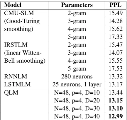
The first experiment consisted in an evaluation of models perplexity (PPL) on the TIMIT testset. We compared the QLM model with two N-gram im-plementations, namely CMU-SLM (Clarkson and Rosenfeld, 1997) and IRSTLM (Federico et al., 2008), and two recurrent NN models able to produce state-of-the-art results in language mod-elling, the RNNLM (Mikolov et al., 2010,2011) and the LSTMLM (Soutner and M¨uller, 2015) packages.

Table1shows the results of the intrinsic evalu-ation. With regard to RNNLM and LSTMLM re-sults, only the best hyper-parameters combination after a lot of experiments, optimizing them on the validation set, has been inserted into the Table.

With regard to QLM, all the presented ex-periments are based on artificial word vectors produced randomly using values from the set

{−1,0,1}instead of real word embeddings. Ev-ery word vector is different from the others and we decided not to use real embeddings in order to test the core QMT method without adding the

contex-Model Parameters PPL

CMU-SLM 2-gram 15.49

(Good-Turing 3-gram 14.28

smoothing) 4-gram 15.62

5-gram 17.33

IRSTLM 2-gram 15.47

(linear Witten- 3-gram 14.07 Bell smoothing) 4-gram 15.55 5-gram 17.53

RNNLM 280 neurons 13.32

LSTMLM 25 neurons, 1 layer 13.17 QLM N=48, p=4, D=10 13.44 N=48, p=4, D=20 13.15 N=48, p=4, D=30 13.10 N=48, p=4, D=40 12.99

Table 1: Perplexity (PPL) of the tested language-modelling techniques on the TIMIT testset. All the QLM results in bold face are better than the other systems we tested.

tual information, contained in word embeddings, that could have helped our approach to obtain bet-ter performances, at least in principle.

5.2.2 Extrinsic evaluation

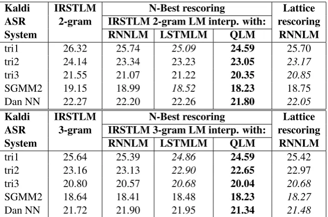
The “TIMIT recipe” contained in the Kaldi dis-tribution2 _{reproduces exactly the same} evalua-tion settings described in (Lopes and Perdigao, 2011) for a phone recognition task based on this corpus. Moreover, Kaldi provides some n-best rescoring scripts that apply RNNLM hypothesis rescoring and interpolate the results with the stan-dard N-gram model results used in the evaluation. We slightly modified these scripts to work with LSTMLM and QLM in order to test different mod-els using the same setting. This allowed us to re-place the LM used in Kaldi and experiment with all the systems evaluated in the previous section.

Table2outlines the results we obtained replac-ing the LM technique into Kaldi ASR package w.r.t. the different ASR systems that the TIMIT recipe implements. These systems are built on top of MFCC, LDA, MLLT, fMLLR with CMN3 fea-tures (see (Povey et al.,2011b;Rath et al.,2013) for all acronyms references and a complete feature

2_{https://github.com/kaldi-asr/kaldi}

3_{MFCC: Mel-Frequency Cepstral Coefficients; LDA:}

or recipe descriptions).

For this extrinsic evaluation we used the best models we obtained in the previous experiments interpolating their log-probability results for each utterance with the original bigram (or trigram) log-probability using a linear model with a ratio 0.25/0.75 between the original N-gram LM and the tested one as suggested in the standard Kaldi rescoring script. For this test we rescored the 10,000-best hypothesis.

We have to say that in this experiment we were not trying to build the best possible phone recog-niser, but simply to compare the relative perfor-mances of the analysed LM techniques showing the effectiveness of QLM when used in a real ap-plication. Thus absolute Phone Error Rate is not so important here and it can be certainly possible to devise recognisers with better performances by applying more sophisticated techniques. For ex-ample (Peddinti et al., 2015) presented a method for lattice rescoring in Kaldi that exhibits better performances than the n-best rescoring we used to interpolate between n-grams and the tested mod-els, but modifying it in order to test LSTMLM and QLM presented a lot of problems and thus we decided to use the simpler n-best approach. For completeness, the last column of Table2 out-lines the results obtained using this lattice rescor-ing method with RNNLM as described in (Ped-dinti et al.,2015).

6 Discussion and conclusions

We presented a new technique for building LM based on QMT, and its probability calculus, test-ing it extensively both with intrinsic and extrinsic evaluation methods.

The PPL results for the intrinsic evaluation, outlined in Table 1, show a clear superiority of the proposed method when compared with state-of-the-art techniques such as RNNLM and LSTMLM. It is interesting to note that even using

D = 20, that means a system containing a quar-ter of paramequar-ters, therefore much less ‘memory’, w.r.t. the system with D = 40, we obtain a PPL performance better than the other methods.

With regard to the second experiment we made, an extrinsic evaluation where we replaced the LM of an ASR system with the LM produced by all the tested methods (see Table 2), QLM consistently exhibits the best performances for all the tested ASR systems from the Kaldi “TIMIT recipe”.

De-spite using a n-best technique in this evaluation for hypothesis rescoring, that is known to perform worse than the lattice rescoring method proposed in (Peddinti et al.,2015), the QLM performances are even better than this method.

The approach we have presented in this paper is not without problems: the number of different word types in the considered language has to be small in order to keep the model computationally tractable. Even if the code we used in the evalu-ations is analytically highly optimised, the train-ing of this model is rather slow and requires rele-vant computational resources even for small prob-lems. On the contrary, inference is very quick, faster than the RNNLM and LSTMLM packages we tested.

The main research question that drove this work was to verify if the distinguishing properties of quantum probability theory, namely interference and system entaglement that could allow the an-cilla to have a “potentially infinite” memory, were enough to build stochastic systems more power-ful than those built using classical probabilities or those built using recurrent NN. Our main aim was not to build a complete model to handle all possible LM scenarios, but to present a “proof-of-concept” study to test the potentialities of this ap-proach. For this reason we tried to keep the model as simple as possible using orthogonal projectors: for measuring probabilities, projecting the system state, each word is mapped onto a single basis vec-tor and the dimension of the system Hilbert space,

N, is equal to the number of different words. Given the matrix dimensions that we have to man-age when we add the ancilla,DN×DN, this set-ting does not scale to real LM problems (e.g. the Brown corpus), even though the calculations are performed usingD×Dsubmatrices, but allowed us to successfully verify the research question. For the same reason out-of-vocabulary words cannot be handled in this model because there are no ba-sis vectors assigned to them.

In order to overcome these limitations, this work can be extended by using generalized quan-tum measurements projectors (POVM) and by us-ing a different structure for the system Hilbert space: instead of mapping each word onto a sin-gle basis vector we can span this space using as basis the samep-basis vectors used to define the

superposi-Kaldi IRSTLM N-Best rescoring Lattice ASR 2-gram IRSTLM 2-gram LM interp. with: rescoring System RNNLM LSTMLM QLM RNNLM

tri1 26.32 25.74 25.09 24.59 25.70

tri2 24.14 23.34 23.23 23.05 23.17

tri3 21.55 21.07 21.22 20.35 20.85

SGMM2 19.15 18.99 18.52 18.23 18.75

Dan NN 22.27 22.20 22.26 21.80 22.05

Kaldi IRSTLM N-Best rescoring Lattice ASR 3-gram IRSTLM 3-gram LM interp. with: rescoring System RNNLM LSTMLM QLM RNNLM

tri1 25.64 25.39 24.86 24.59 25.42

tri2 23.16 23.13 22.90 22.65 22.97

tri3 20.80 20.57 20.68 20.04 20.68

SGMM2 18.64 18.41 18.48 18.23 18.27

Dan NN 21.72 21.90 21.95 21.34 21.48

Table 2: Phone-recognition performances, in terms of Phone Error Rate, for the TIMIT dataset and the different Kaldi ASR models, rescoring the 10,000-best solutions with the tested LM techniques in-terpolated with the IRSTLM bigrams and trigrams LM (the standard LM used in Kaldi). In boldface the best performing system and in italics the second best. Kaldi ASR systems descriptions: tri1 = a triphone model using 13 dim. MFCC+∆+∆∆; tri2 = tri1+LDA+MLLT; tri3 = tri2+SAT; SGMM2 = Semi-supervised Gaussian Mixture Model (Huang and Hasegawa-Johnson,2010;Povey et al.,2011a); Dan NN = DNN model by (Zhang et al.,2014;Povey et al.,2015).

tion on thep-basis. Such improvement would re-duce dramatically the dimensions of the matrices toDp ×Dp potentially mitigating the computa-tional issue. Moreover, this would solve also the problem of out-of-vocabulary words allowing for a proper management of the large set of different words typical of real applications.

We are still working on these improvements and we will hope to get a complete model soon.

With this contribution we would like to raise also some interest in the community to analyse and develop more effective techniques, both on the modelling and minimisation/learning sides, to allow to build real world application based on this framework. QMT and its probability calculus seem to be promising methodologies to enhance the performances of our systems in NLP and cer-tainly deserve further investigations.

Acknowledgments

We acknowledge the CINECA4 _{award no.} HP10C7XVUO under the ISCRA initiative, for the availability of HPC resources and support.

4_{https://www.cineca.it/en}

References

Diederik Aerts, Jan Broekaert, Liane Gabora, and Sandro Sozzo. 2013. Quantum structure and hu-man thought. Behavioral and Brain Sciences, 36(3):274276.

Martin Arjovsky, Amar Shah, and Yoshua Bengio. 2016. Unitary evolution recurrent neural networks. InProceedings of the 33rd International Conference on International Conference on Machine Learning -ICML’16, pages 1120–1128.

Yoshua Bengio. 2012. Practical recommendations for gradient-based training of deep architectures. In Gr´egoire Montavon, Genevi`eve B. Orr, and Klaus-Robert M¨uller, editors,Neural Networks: Tricks of the Trade: Second Edition, pages 437–478. Springer Berlin Heidelberg, Berlin, Heidelberg.

William Blacoe, Elham Kashefi, and Mirella Lapata. 2013. A quantum-theoretic approach to distribu-tional semantics. In Proceedings of Human Lan-guage Technologies: Conference of the North Amer-ican Chapter of the Association of Computational Linguistics, Atlanta, Georgia, pages 847–857.

Jerome R. Busemeyer and Peter D. Bruza. 2012. Quan-tum Models of Cognition and Decision. Cambridge University Press, New York, NY.

toolkit. In Proceedings of EUROSPEECH ’97, pages 2707–2710. ISCA.

Marcello Federico, Nicola Bertoldi, and Mauro Cet-tolo. 2008. IRSTLM: an open source toolkit for handling large scale language models. In INTER-SPEECH 2008, 9th Annual Conference of the Inter-national Speech Communication Association, Bris-bane, Australia, pages 1618–1621.

John Garofolo, Lori Lamel, William Fisher, Jonathan Fiscus, David Pallett, Nancy Dahlgren, and Vic-tor Zue. 1990. Darpa timit acoustic-phonetic con-tinuous speech corpus cd-rom. DARPA, TIMIT Acoustic-Phonetic Continuous Speech Corpus CD-ROM.

Fabio A. Gonz´alez and Juan C. Caicedo. 2011. Quan-tum latent semantic analysis. InAdvances in Infor-mation Retrieval Theory, LNCS, 6931, pages 52–63. Jui Ting Huang and Mark Hasegawa-Johnson. 2010. Semi-supervised training of gaussian mixture mod-els by conditional entropy minimization. In Pro-ceedings of the 11th Annual Conference of the In-ternational Speech Communication Association, IN-TERSPEECH 2010, pages 1353–1356.

Li Jing, Yichen Shen, Tena Dubcek, John Peurifoy, Scott A. Skirlo, Max Tegmark, and Marin Soljacic. 2017. Tunable efficient unitary neural networks (EUNN) and their application to RNN. In Thirty-fourth International Conference on Machine Learn-ing - ICML2017.

Dimitrios Kartsaklis, Martha Lewis, and Laura Rimell. 2016.Proceedings of the 2016 Workshop on Seman-tic Spaces at the Intersection of NLP, Physics and Cognitive Science, volume 221. Electronic Proceed-ings in Theoretical Computer Science.

Andrei Y. Khrennikov. 2010. Ubiquitous Quantum Structure: From Psychology to Finance. Springer-Verlag Berlin Heidelberg.

Ding Liu, Xiaofang Yang, and Minghu Jiang. 2013. A novel classifier based on quantum computation. In Proceedings of the 51st Annual Meeting of the As-sociation for Computational Linguistics, Sofia, Bul-garia, pages 484–488.

Carla Lopes and Fernando Perdigao. 2011. Phoneme recognition on the timit database. In Ivo Ipsic, edi-tor,Speech Technologies. InTech, Rijeka.

Massimo Melucci. 2015. Introduction to Information Retrieval and Quantum Mechanics. The Informa-tion Retrieval Series 35. Springer-Verlag Berlin Hei-delberg.

Massimo Melucci and Keith van Rijsbergen. 2011. Quantum mechanics and information retrieval. In Massimo Melucci and Ricardo Baeza-Yates, editors, Advanced Topics in Information Retrieval, pages 125–155. Springer Berlin Heidelberg, Berlin, Hei-delberg.

Tomas Mikolov, Kai Chen, Greg Corrado, and Jeffrey Dean. 2013. Efficient Estimation of Word Repre-sentations in Vector Space. InProc. of Workshop at ICLR.

Tomas Mikolov, Martin Karafi´at, Luk´as Burget, Jan Cernock´y, and Sanjeev Khudanpur. 2010. Recur-rent neural network based language model. In IN-TERSPEECH 2010, 11th Annual Conference of the International Speech Communication Association, Makuhari, Chiba, Japan, pages 1045–1048.

Tom´aˇs Mikolov, Stefan Kombrink, Anoop Deoras, Luk´aˇs Burget, and Jan ˇCernock´y. 2011. Rnnlm -recurrent neural network language modeling toolkit. InProceedings of ASRU 2011, pages 1–4.

Jorge J. Mor´e and David J. Thuente. 1994. Line search algorithms with guaranteed sufficient de-crease. ACM Trans. Math. Softw., 20(3):286–307.

Michael A. Nielsen and Isaac L. Chuang. 2010. Quan-tum Computation and QuanQuan-tum Information: 10th Anniversary Edition. Cambridge University Press.

J. Nocedal and S. J. Wright. 2006. Numerical Opti-mization, 2nd edition. Springer, New York.

Vijayaditya Peddinti, Guoguo Chen, Vimal Manohar, Tom Ko, Daniel Povey, and Sanjeev Khudanpur. 2015. JHU aspire system: Robust LVCSR with tdnns, ivector adaptation and RNN-LMS. In2015 IEEE Workshop on Automatic Speech Recognition and Understanding, ASRU 2015, Scottsdale, AZ, USA, pages 539–546.

Daniel Povey, Luk´aˇs Burget, Mohit Agarwal, Pinar Akyazi, Feng Kai, Arnab Ghoshal, Ondˇrej Glem-bek, Nagendra Goel, Martin Karafi´at, Ariya Ras-trow, Richard C. Rose, Petr Schwarz, and Samuel Thomas. 2011a. The subspace gaussian mixture model-a structured model for speech recognition. Comput. Speech Lang., 25(2):404–439.

Daniel Povey, Arnab Ghoshal, Gilles Boulianne, Lukas Burget, Ondrej Glembek, Nagendra Goel, Mirko Hannemann, Petr Motlicek, Yanmin Qian, Petr Schwarz, Jan Silovsky, Georg Stemmer, and Karel Vesely. 2011b. The kaldi speech recognition toolkit. In IEEE 2011 Workshop on Automatic Speech Recognition and Understanding. IEEE Signal Pro-cessing Society.

Daniel Povey, Xiaohui Zhang, and Sanjeev Khudanpur. 2015. Parallel training of dnns with natural gradient and parameter averaging. InInternational Confer-ence on Learning Representations - ICLR2015.

Shakti P. Rath, Daniel Povey, Karel Vesel´y, and Jan Cernock´y. 2013. Improved feature processing for deep neural networks. In Proceedings of the 14th Annual Conference of the International Speech Communication Association - INTERSPEECH2013, Lyon, France, pages 109–113.

Daniel Soutner and Ludˇek M¨uller. 2015. In Adrian-Horia Dediu, Carlos Mart´ın-Vide, and Kl´ara Vicsi, editors, Statistical Language and Speech Process-ing: Third International Conference, SLSP 2015, Budapest, Hungary, November 24-26, 2015, Pro-ceedings, pages 267–274. Springer International Publishing.

Christoph Spengler, Marcus Huber, and Beatrix C Hiesmayr. 2010. A composite parameterization of unitary groups, density matrices and subspaces. Journal of Physics A: Mathematical and Theoreti-cal, 43(38):385306.

H.D. Tagare. 2011. Notes on optimization on Stiefel manifolds. Technical report, Technical report, Yale University.

Fabio Tamburini. 2014. Are quantum classifiers promising? InProceedings of the First Italian Con-ference on Computational Linguistics CLiC-it 2014, Pisa, Pisa University Press, pages 360–364. Vlatko Vedral. 2007. Introduction to Quantum

Infor-mation Science. Oxford University Press, USA. Scott Wisdom, Thomas Powers, John Hershey,

Jonathan Le Roux, and Les Atlas. 2016. Full-capacity unitary recurrent neural networks. In D. D. Lee, M. Sugiyama, U. V. Luxburg, I. Guyon, and R. Garnett, editors,Advances in Neural Information Processing Systems 29, pages 4880–4888. Curran Associates, Inc.

Xiaohui Zhang, Jan Trmal, Daniel Povey, and San-jeev Khudanpur. 2014. Improving deep neural work acoustic models using generalized maxout net-works. InAcoustics, Speech and Signal Processing (ICASSP), 2014 IEEE International Conference on, pages 215–219. IEEE.