Efficient Attention using a Fixed Size Memory Representation

Efficient Attention using a Fixed-Size Memory Representation

Denny Britz∗_{and Melody Y. Guan}∗_{and Minh-Thang Luong}

Google Brain

dennybritz,melodyguan,[email protected]

Abstract

The standard content-based attention mecha-nism typically used in sequence-to-sequence models is computationally expensive as it requires the comparison of large encoder and decoder states at each time step. In this work, we propose an alternative attention mechanism based on a fixed size memory representation that is more efficient. Our technique predicts a compact set of K

attention contexts during encoding and lets the decoder compute an efficient lookup that does not need to consult the memory. We show that our approach performs on-par with the standard attention mechanism while yielding inference speedups of 20% for real-world translation tasks and more for tasks with longer sequences. By visualizing attention scores we demonstrate that our models learn distinct, meaningful alignments. 1 Introduction

Sequence-to-sequence models (Sutskever et al.,

2014;Cho et al., 2014) have achieved state of the art results across a wide variety of tasks, including Neural Machine Translation (NMT) (Bahdanau et al.,

2014;Wu et al.,2016), text summarization (Rush et al.,2015;Nallapati et al.,2016), speech recognition (Chan et al.,2015;Chorowski and Jaitly,2016), image captioning (Xu et al., 2015), and conversational modeling (Vinyals and Le,2015;Li et al.,2015).

The most popular approaches are based on an encoder-decoder architecture consisting of two recurrent neural networks (RNNs) and an attention mechanism that aligns target to source tokens ( Bah-danau et al.,2014;Luong et al.,2015). The typical attention mechanism used in these architectures computes a new attention context at each decoding

∗_{Equal Contribution. Author order alphabetical.}

step based on the current state of the decoder. Intuitively, this corresponds to looking at the source sequence after the output of every single target token.

Inspired by how humans process sentences, we believe it may be unnecessary to look back at the entire original source sequence at each step.1_{We thus}

propose an alternative attention mechanism (section3) that leads to smaller computational time complexity. Our method predictsKattention context vectors while reading the source, and learns to use a weighted av-erage of these vectors at each step of decoding. Thus, we avoid looking back at the source sequence once it has been encoded. We show (section4) that this speeds up inference while performing on-par with the standard mechanism on both toy and real-world WMT translation datasets. We also show that our mecha-nism leads to larger speedups as sequences get longer. Finally, by visualizing the attention scores (section

5), we verify that the proposed technique learns mean-ingful alignments, and that different attention context vectors specialize on different parts of the source. 2 Background

2.1 Sequence-to-Sequence Model with Attention Our models are based on an encoder-decoder archi-tecture with attention mechanism (Bahdanau et al.,

2014;Luong et al.,2015). An encoder function takes as input a sequence of source tokensx=(x1,...,xm)

and produces a sequence of statess=(s1,...,sm).The

decoder is an RNN that predicts the probability of a target sequencey=(y1,...,yT|s). The probability of

each target tokenyi∈ {1,...,|V|}is predicted based

on the recurrent state in the decoder RNN,hi, the

pre-vious words,y<i, and a context vectorci. The context

vectorci, also referred to as the attention vector, is

calculated as a weighted average of the source states.

1_{Eye-tracking and keystroke logging data from human}

translators show that translators generally do not reread previously translated source text words when producing target text (Carl et al.,2011).

ci= X

j

αijsj (1)

αi=softmax(fatt(hi,s)) (2)

Here, fatt(hi,s) is an attention function that

calculates an unnormalized alignment score between the encoder statesjand the decoder statehi. Variants

offattused in Bahdanau et al.(2014) and Luong et al.(2015) are:

fatt(hi,sj)= (

vT

atanh(Wa[hi,sj]), Bahdanau hT

i Wasj Luong

whereWaandvaare model parameters learned to

predict alignment. Let|S|and|T|denote the lengths of the source and target sequences respectively andD

denoate the state size of the encoder and decoder RNN. Such content-based attention mechanisms result in in-ference times ofO(D2_|S||T|)2_{, as each context vector}

depends on the current decoder statehiand all encoder

states, and requires anO(D2_{)matrix multiplication.} The decoder outputs a distribution over a vocabulary of fixed-size|V|:

P(yi|y<i,x)=softmax(W[si;ci]+b) (3)

The model is trained end-to-end by minimizing the negative log likelihood of the target words using stochastic gradient descent.

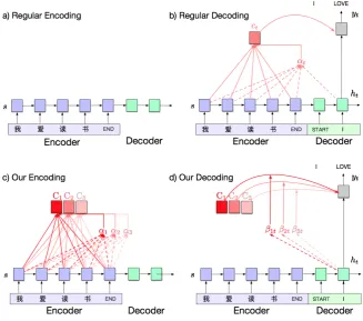
3 Memory-Based Attention Model

Our proposed model is shown in Figure1. During en-coding, we compute an attention matrixC∈RK×D_,

where K is the number of attention vectors and a hyperparameter of our method, andDis the dimen-sionality of the top-most encoder state. This matrix is computed by predicting a score vectorαt∈RK

at each encoding time step t. C is then a linear combination of the encoder states, weighted byαt:

Ck= |S| X

t=0

αtkst (4)

αt=softmax(Wαst), (5)

whereWαis a parameter matrix inRK×D.

The computational time complexity for this operation is O(KD|S|). One can think of C as compact fixed-length memory that the decoder

2_{An exception is the dot-attention from Luong et al.(2015),}

which isO(D|S||T|), which we discuss further in Section 3.

will perform attention over. In contrast, standard approaches use a variable-length set of encoder states for attention. At each decoding step, we similarly predictKscoresβ∈RK_{. The final attention context} cis a linear combination of the rows inCweighted by the scores. Intuitively, each decoder step predicts how important each of theKattention vectors is.

c=XK

i=0

βiCi (6)

β=softmax(Wβh) (7)

Here,his the current state of the decoder, andWβis a

learned parameter matrix. Note that we do not access the encoder states at each decoder step. We simply take a linear combination of the attention matrixC

pre-computed during encoding - a much cheaper op-eration that is independent of the length of the source sequence. The time complexity of this computation isO(KD|T|)as multiplication with theKattention matrices needs to happen at each decoding step.

Summing O(KD|S|) from encoding and

O(KD|T|) from decoding, we have a total linear computational complexity of O(KD(|S| + |T|). As Dis typically very large, 512or 1024units in most applications, we expect our model to be faster than the standard attention mechanism running in

O(D2_{|S||T|). For long sequences (as in} summariza-tion, where —S— is large), we also expect our model to be faster than the cheaper dot-based attention mech-anism, which needsO(D|S||T|) computation time and requires encoder and decoder states sizes to match. We also experimented with using a sigmoid function instead of the softmax to score the encoder and decoder attention scores, resulting in 4 possible combinations. We call this choice thescoring function. A softmax scoring function calculates normalized scores, while the sigmoid scoring function results in unnormalized scores that can be understood as gates. 3.1 Model Interpretations

Figure 1: Memory Attention model architecture. K attention vectors are predicted during encoding, and a linear combination is chosen during decoding. In our example,K=3.

a regular attention model and adding a regularization term to force the memory matrix C to be close to theT×Dvectors computed by the standard attention. We leave it to future work to explore such an objective. Alternatively, we can interpret our mechanism as first predicting a compactK×Dmemory matrix, a representation of the source sequence, and then performinglocation-basedattention on the memory by picking which row of the matrix to attend to. Standard location-based attention mechanism, by contrast, predicts a location in the source sequence to focus on (Luong et al.,2015;Xu et al.,2015).

3.2 Position Encodings (PE)

In the above formulation, the predictions of attention contexts are symmetric. That is,Ci is not forced to

be different fromCj6=i. While we would hope for the

model to learn to generate distinct attention contexts, we now present an extension that pushes the model into this direction. We addposition encodingsto the score matrix that forces the first few context vector

C1,C2,...to focus on the beginning of the sequence and the last few vectors...,CK−1,CKto focus on the

end (thereby encouraging in-between vectors to focus on the middle).

Explicitly, we multiply the score vector α with

position encodingsls∈RK:

CPE=

|S| X

s=0

αPEhs (8)

αPE_s =softmax(Wαhs◦ls) (9)

To obtainlswe first calculate a constant matrixL

where we define each element as

Lks=(1−k/K)(1−s/S)+_Kk _Ss, (10)

Figure 2: Surface for the position encodings.

4 Experiments

4.1 Toy Copying Experiment

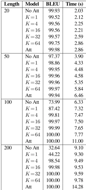
Due to the reduction of computational time complex-ity we expect our method to yield performance gains especially for longer sequences and tasks where the source can be compactly represented in a fixed-size memory matrix. To investigate the trade-off between speed and performance, we compare our technique to standard models with and without attention on a Sequence Copy Task of varying length like inGraves et al.(2014). We generated 4 training datasets of 100,000 examples and a validation dataset of 1,000 ex-amples. The vocabulary size was 20. For each dataset, the sequences had lengths randomly chosen between 0 toL, forL∈{10,50,100,200}unique to each dataset. 4.1.1 Training Setup

All models are implemented using TensorFlow based on the seq2seq implementation of Britz et al.

(2017)3 _{and trained on a single machine with a}

Nvidia K40m GPU. We use a 2-layer 256-unit, a bidirectional LSTM (Hochreiter and Schmidhuber,

1997) encoder, a 2-layer 256-unit LSTM decoder, and 256-dimensional embeddings. For the attention baseline, we use the standard parametrized attention (Bahdanau et al., 2014). Dropout of 0.2 (0.8 keep probability) is applied to the input of each cell and we optimize using Adam (Kingma and Ba,2014) at a learning rate of 0.0001 and batch size 128. We train for at most 200,000 steps (see Figure3for sample learning curves). BLEU scores are calculated on tokenized data using the multi-bleu.perl script in Moses.4_{We decode using beam search with a beam}

3_{http://github.com/google/seq2seq}

4_{http://github.com/moses-smt/mosesdecoder}

Length Model BLEU Time (s) 20 No Att 99.93 2.03

K=1 99.52 2.12

K=4 99.56 2.25

K=16 99.56 2.21

K=32 99.57 2.59

K=64 99.75 2.86 Att 99.98 2.86 50 No Att 97.37 3.90

K=1 98.86 4.33

K=4 99.95 4.48

K=16 99.96 4.58

K=32 99.96 5.35

K=64 99.97 5.84 Att 99.94 6.46 100 No Att 73.99 6.33

K=1 87.42 7.32

K=4 99.81 7.47

K=16 99.97 7.50

K=32 99.99 7.65

K=64 100.00 7.77 Att 100.00 11.00 200 No Att 32.64 9.10

K=1 44.22 9.30

K=4 98.54 9.49

K=16 99.98 9.53

K=32 100.00 9.59

K=64 100.00 9.78 Att 100.00 14.28

Table 1: BLEU scores and computation times with varyingKand sequence length compared to baseline models with and without attention.

size of 10 (Wiseman and Rush,2016).

4.1.2 Results

0 50 100 150 200 steps (k)

0.0 0.5 1.0 1.5 2.0 2.5 3.0 3.5

log perplexity

K=1 K=4 K=16 K=32 K=64 attention no attention

(a) Comparison of varyingKfor copying sequences of length 200 on evaluation data, showing that largeK leads to faster convergence and smallKperforms similarly to the non-attentional baseline.

0 50 100 150 200 steps (k)

0.0 0.5 1.0 1.5 2.0 2.5 3.0 3.5

log perplexity

sigmoid/sigmoid sigmoid/softmax softmax/sigmoid softmax/softmax

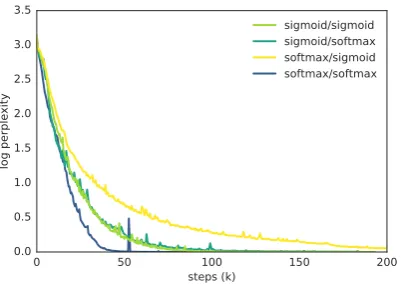
(b) Comparison of sigmoid and softmax functions for choosing the encoder and decoder attention scores on evaluation data, showing that choice of gating/normalization matters.

Figure 3: Training Curves for the Toy Copy task

That we are able to represent the source sequence with a fixed size matrix with fewer than |S| rows suggests that traditional attention mechanisms may be representing the source with redundancies and wasting computational resources. This makes intuitive sense for the toy task, which should require a relatively simple representation.

The last column shows that our technique signif-icantly speeds up the inference process. The gap in inference speed increases as sequences become longer. We measured inference time on the full validation set of 1,000 examples, not including data loading or model construction times.

Figure3ashows the learning curves for sequence length 200. We see thatK=1is unable to fit the data distribution, whileK∈{32,64}fits the data almost as quickly as the attention-based model. Figure3bshows the effect of varying the encoder and decoder scoring functions between softmax and sigmoid. All combina-tions manage to fit the data, but some converge faster than others. In section5we show that distinct align-ments are learned by different function combinations. 4.2 Machine Translation

Next, we explore if the memory-based attention mechanism is able to fit complex real-world datasets. For this purpose we use 4 large machine translation datasets of WMT’175 _{on the following language}

pairs: Czech (en-cs, 52M examples), English-German (en-de, 5.9M examples), English-Finish (en-fi, 2.6M examples), and English-Turkish (en-tr, 207,373 examples). We used the newly available

pre-5_{statmt.org/wmt17/translation-task.html}

processed datasets for the WMT’17 task.6_{Note that}

our scores may not be directly comparable to other work that performs their own data pre-processing. We learn shared vocabularies of 16,000 subword units using the BPE algorithm (Sennrich et al., 2016). We use newstest2015 as a validation set, and report BLEU on newstest2016.

4.2.1 Training Setup

We use a similar setup to the Toy Copy task, but use 512 RNN and embedding units, train using 8 distributed workers with 1 GPU each, and train for at most 1M steps. We save checkpoints every 30 minutes during training, and choose the best based on the validation BLEU score.

4.2.2 Results

Table 2 compares our approach with and without position encodings, and with varying values for hyperparameterK, to baseline models with regular attention mechanism. Learning curves are shown in Figure4. We see that our memory attention model with sufficiently high K performs on-par with, or slightly better, than the attention-based baseline model despite its simpler nature. Across the board, models with K = 64performed better than corresponding models withK= 32, suggesting that using a larger number of attention vectors can capture a richer under-standing of source sequences. Position encodings also seem to consistently improve model performance.

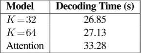
Table3shows that our model results in faster de-coding time even on a complex dataset with a large

K K

(a) Training curves for en-fi

K K

(b) Training curves for en-tr

Figure 4: Comparing training curves for en-fi and en-tr with sigmoid encoder scoring and softmax decoder scoring and position encoding. Note that en-tr curves converged very quickly.

Model Dataset K en-cs en-de en-fi en-tr Memory Attention Test 32 19.37 28.82 15.87

-64 19.65 29.53 16.49 -Valid 32 19.20 26.20 15.90 12.94

64 19.63 26.39 16.35 13.06 Memory Attention + PE Test 32 19.45 29.53 15.86

-64 20.36 30.61 17.03 -Valid 32 19.35 26.22 16.31 12.97

64 19.73 27.31 16.91 13.25 Attention Test - 19.19 30.99 17.34

-Valid - 18.61 28.13 17.16 13.76

Table 2: BLEU scores on WMT’17 translation datasets from the memory attention models and regular attention baselines. We picked the best out of the four scoring function combinations on the validation set. Note that en-tr does not have an official test set. Best test scores on each dataset are highlighted.

Model Decoding Time (s)

K=32 26.85

K=64 27.13

Attention 33.28

Table 3: Decoding time, averaged across 10 runs, for the en-de validation set (2169 examples) with average sequence length of 35. Results are similar for both PE and non-PE models.

vocabulary of 16k. We measured decoding time over the full validation set, not including time used for model setup and data loading, averaged across 10 runs. The average sequence length for examples in this data was 35, and we expect more significant speedups for tasks with longer sequences, as suggested by our experiments on toy data. Note that in our NMT

ex-amples/experiments,K≈T, but we obtain computa-tional savings from the fact thatKD. We may be able to setKT, as in toy copying, and still get very good performance in other tasks. For instance, in sum-marization the source is complex but the representa-tion of the source required to perform the task is ”sim-ple” (i.e. all that is needed to generate the abstract).

K K K K

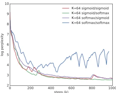
Figure 5: Comparing training curves for en-fi for different encoder/decoder scoring functions for our models atK=64.

5 Visualizing Attention

A useful property of the standard attention mechanism is that it produces meaningful alignment between source and target sequences. Often, the attention mechanism learns to progressively focus on the next source token as it decodes the target. These visualizations can be an important tool in debugging and evaluating seq2seq models and are often used for unknown token replacement.

This raises the question of whether or not our proposed memory attention mechanism also learns to generate meaningful alignments. Due to limiting the number of attention contexts to a number that is generally less than the sequence length, it is not immediately obvious what each context would learn to focus on. Our hope was that the model would learn to focus on multiple alignments at the same time, within the same attention vector. For example, if the source sequence is of length 40 and we haveK=10

attention contexts, we would hope thatC1roughly fo-cuses on tokens 1 to 4,C2on tokens 5 to 8, and so on. Figures6and7show that this is indeed the case. To generate this visualization we multiply the attention scoresαandβfrom the encoder and decoder. Figure

8shows a sample translation task visualization. Figure 6 suggests that our model learns distinct ways to use its memory depending on the encoder and decoder functions. Interestingly, using softmax nor-malization results in attention maps typical of those de-rived from using standard attention, i.e. a relatively lin-ear mapping between source and target tokens. Mean-while, using sigmoid gating results in what seems to be a distributed representation of the source sequences across encoder time steps, with multiple contiguous at-tention contexts being accessed at each decoding step.

6 Related Work

Our contributions build on previous work in making seq2seq models more computationally efficient.

Luong et al.(2015) introduce various attention mech-anisms that are computationally simpler and perform as well or better than the original one presented in

Bahdanau et al.(2014). However, these typically still requireO(D2_{)computation complexity, or lack the} flexibility to look at the full source sequence. Efficient location-based attention (Xu et al.,2015) has also been explored in the image recognition domain.

Wu et al.(2016) presents several enhancements to the standard seq2seq architecture that allow more effi-cient computation on GPUs, such as only attending on the bottom layer. Kalchbrenner et al.(2016) propose a linear time architecture based on stacked convolu-tional neural networks. Gehring et al.(2016) also propose the use of convolutional encoders to speed up NMT. de Br´ebisson and Vincent(2016) propose a lin-ear attention mechanism based on covariance matrices applied to information retrieval. Raffel et al.(2017) enable online linear time attention calculation by en-forcing that the alignment between input and output sequence elements be monotonic. Previously, mono-tonic attention was proposed for morphological inflec-tion generainflec-tion by Aharoni and Goldberg(2016). 7 Conclusion

Figure 6: Attention scores at each step of decoding for on a sample from the sequence length 100 toy copy dataset. Individual attention vectors are highlighted in blue. (y-axis: source tokens;x-axis: target tokens)

K K K K

Figure 7: Attention scores at each step of decoding forK= 4on a sample with sequence length 11. The subfigure on the left color codes each individual attention vector. (y-axis: source;x-axis: target)

C1 C2 C3 C4 C5 C6 C7 C8

C9 C10 C11 C12 C13 C14 C15 C16

C17 C18 C19 C20 C21 C22 C23 C24

C25 C26 C27 C28 C29 C30 C31 C32

References

Roee Aharoni and Yoav Goldberg. 2016.

Mor-phological inflection generation with hard monotonic attention. CoRR abs/1611.01487. http://arxiv.org/abs/1611.01487.

Dzmitry Bahdanau, Kyunghyun Cho, and Yoshua Bengio. 2014. Neural machine translation by jointly learning to align and translate. CoRRabs/1409.0473. http://arxiv.org/abs/1409.0473.

Denny Britz, Anna Goldie, Thang Luong, and Quoc Le. 2017. Massive Exploration of Neural Machine Translation Architectures. CoRR abs/1703.03906. http://arxiv.org/abs/1703.03906.

Michael Carl, Barbara Dragsted, and Arnt Lykke Jakob-sen. 2011. A taxonomy of human translation styles.

Translation Journal16(2).

William Chan, Navdeep Jaitly, Quoc V. Le, and Oriol Vinyals. 2015. Listen, attend and spell. CoRR

abs/1508.01211.http://arxiv.org/abs/1508.01211. Kyunghyun Cho, Bart van Merrienboer, C¸aglar G¨ulc¸ehre,

Fethi Bougares, Holger Schwenk, and Yoshua Bengio. 2014. Learning phrase representations using RNN encoder-decoder for statistical machine translation. In

EMNLP.

Jan Chorowski and Navdeep Jaitly. 2016. Towards better decoding and language model integration in sequence to sequence models. CoRRabs/1612.02695. http://arxiv.org/abs/1612.02695.

Alexandre de Br´ebisson and Pascal Vincent. 2016. A cheap linear attention mechanism with fast lookups and fixed-size representations. CoRRabs/1609.05866. http://arxiv.org/abs/1609.05866.

Jonas Gehring, Michael Auli, David Grangier, and Yann N. Dauphin. 2016. A convolutional encoder model for neural machine translation. CoRR abs/1611.02344. http://arxiv.org/abs/1611.02344.

Alex Graves, Greg Wayne, and Ivo Danihelka. 2014. Neural turing machines. CoRR abs/1410.5401. http://arxiv.org/abs/1410.5401.

Sepp Hochreiter and J¨urgen Schmidhuber. 1997. Long short-term memory. Neural Computation 9(8):1735– 1780.

Nal Kalchbrenner, Lasse Espeholt, Karen Simonyan, A¨aron van den Oord, Alex Graves, and Koray

Kavukcuoglu. 2016. Neural machine

trans-lation in linear time. CoRR abs/1610.10099. http://arxiv.org/abs/1610.10099.

Diederik P. Kingma and Jimmy Ba. 2014. Adam: A method for stochastic optimization. CoRR

abs/1412.6980. http://arxiv.org/abs/1412.6980. Jiwei Li, Michel Galley, Chris Brockett, Jianfeng Gao,

and Bill Dolan. 2015. A diversity-promoting objective function for neural conversation models. CoRR

abs/1510.03055.http://arxiv.org/abs/1510.03055.

Minh-Thang Luong, Hieu Pham, and Christopher D. Man-ning. 2015. Effective approaches to attention-based neural machine translation. CoRR abs/1508.04025. http://arxiv.org/abs/1508.04025.

Ramesh Nallapati, Bing Xiang, and Bowen

Zhou. 2016. Sequence-to-sequence rnns for text summarization. CoRR abs/1602.06023. http://arxiv.org/abs/1602.06023.

Colin Raffel, Thang Luong, Peter J. Liu, Ron J. Weiss, and Douglas Eck. 2017. Online and linear-time attention by enforcing monotonic alignments. CoRR

abs/1704.00784.http://arxiv.org/abs/1704.00784. Alexander M. Rush, Sumit Chopra, and Jason Weston.

2015. A neural attention model for abstractive sentence summarization. CoRR abs/1509.00685. http://arxiv.org/abs/1509.00685.

Rico Sennrich, Barry Haddow, and Alexandra Birch. 2016. Neural machine translation of rare words with subword units. InACL.

Sainbayar Sukhbaatar, Arthur Szlam, Jason We-ston, and Rob Fergus. 2015. Weakly super-vised memory networks. CoRR abs/1503.08895. http://arxiv.org/abs/1503.08895.

Ilya Sutskever, Oriol Vinyals, and Quoc V. Le. 2014. Sequence to sequence learning with neural networks. InNIPS.

Oriol Vinyals and Quoc V. Le. 2015. A neural conversational model. CoRR abs/1506.05869. http://arxiv.org/abs/1506.05869.

Sam Wiseman and Alexander M. Rush. 2016. Sequence-to-sequence learning as beam-search optimization. CoRR abs/1606.02960. http://arxiv.org/abs/1606.02960.

Yonghui Wu, Mike Schuster, Zhifeng Chen, Quoc V. Le, Mohammad Norouzi, Wolfgang Macherey, Maxim Krikun, Yuan Cao, Qin Gao, Klaus Macherey, Jeff Klingner, Apurva Shah, Melvin Johnson, Xiaobing Liu, Lukasz Kaiser, Stephan Gouws, Yoshikiyo Kato, Taku Kudo, Hideto Kazawa, Keith Stevens, George Kurian, Nishant Patil, Wei Wang, Cliff Young, Jason Smith, Ja-son Riesa, Alex Rudnick, Oriol Vinyals, Greg Corrado, Macduff Hughes, and Jeffrey Dean. 2016. Google’s neural machine translation system: Bridging the gap between human and machine translation. CoRR

abs/1609.08144.http://arxiv.org/abs/1609.08144. Kelvin Xu, Jimmy Ba, Ryan Kiros, Kyunghyun