Abstract—This paper presents a systematic methodology for analyzing the maintenance data of offshore system to gain insight about the system reliability performance and identify the critical factors influencing the performance. The study approach is based on problem and data-led rather than technique-driven. The results of trend test propose that the system under studied can be modeled using a simple Homogeneous Poisson process (HPP) where the failure rate is constant. Analyses of covariates are done using Kaplan Meier and Proportional hazards models. The results indicate that the preventive maintenance (PM) plus engine wash has a significance positive influence on the system failure distribution.
Index Terms— HPP, Kaplan Meier, Proportional hazards model, Trend test.
I. INTRODUCTION
The details and statistics of equipment performance in the plant are mostly stored in the maintenance record, and these include the frequency and time of failures, shutdown duration, failure breakdown, types of mitigation and details of scheduled maintenance. Proper, reliable and systematic maintenance record is vital for the sustenance of high standard maintenance practice and the successful of equipment failure analysis or troubleshooting activities. Another benefit of maintenance data which is generally untapped is its potential to provide understanding of the system performance level and assistance in decision making. Maintenance data with proper statistical analysis techniques can help management to assess plant performance by giving insights on how well the performance of the existing system and what critical factors influencing the system performance [1].
An effective analysis of maintenance data requires a systematic approach in which skill, experience and care are the utmost importance for success [2]. Nevertheless, a systematic approach has few salient elements. The first one is a clear objective. The analysis should be based on a clear objective since the objective will set the proper approach in the whole aspects of analysis process. The collection of right data in an appropriate format is fundamental in development of model and subsequent prediction based on that model. Many issues in the data gathering and subsequent analysis processes can be related to the lack of clear objectives at the beginning of data collection process [2]. Poor data will lead to incorrect assumptions and hence produces error in estimates. Next, the analysis approach should be problem-led and data driven rather than technique-driven. Many approaches
Manuscript received Nov 20, 2009. H. Hussin, F.M. Hashim and M. Muhammad are with the Mechanical Engineering Department, Universiti Teknologi Petronas, Bandar Seri Iskandar, 31750, Perak, Malaysia. (corresponding e-mail: [email protected]). S. N. Ibrahim is with Petronas Carigali Sdn. Bhd. (e-mail: [email protected]).
however are more towards techniques-driven which produce outcomes that neither addressing the problem nor practical for implementation in real industry. The technique-driven approach also tends to make a general assumption about the failure model (i.e. most common is constant failure rate) without first conducting proper data analysis in order to legitimate the use of certain technique in the analysis. In many cases, such assumption may not be true thus the results produced will be inaccurate. It is also common to find many research papers on maintenance data analysis focusing too much on mathematical modeling rather than solution to the problems [3]. The problem with this approach is that it will make it difficult for practitioners to grasp the idea and interpret the analysis process due to their incompetence in complex mathematics. Lastly, the analysis should be conducted first by using a simple model before extending it into a more complex model [1]. There is a tendency to apply complex techniques for solving plant problems where in many times these problems can be solved simply by using fairly simple models. The assumption of simpler model to describe the maintenance data can only be rejected when there is enough evidence that the model is inappropriate.
The objective of this study is to present a methodology to systematically analyze the maintenance data to gain insight about the system performance and identify the critical factors influencing that performance. In this study, a practical step-by-step analysis based on problem-led approach is employed. Suitable techniques and models are explored and used based on the finding from the previous steps.
II. MODELS FOR A REPAIRABLE SYSTEM
Most of the equipment on offshore platforms are repairable items, which means that upon failures the equipment are repaired and restored to the functional state. By contrast, non-repairable items are replaced or discarded when they fail. The probabilistic model for studying the occurrence of failures in the repairable system is based on stochastic point processes. The point process can be described as the occurrence of randomly distributed events in time with negligible events duration [4]. The events here are the failure times of a repairable item. Several point process models for repairable system are proposed in the literature and they generally can be classified under three types of repair actions; perfect repair, minimal repair and imperfect repair [5].
In the perfect repair model, the equipment upon failure is either repaired or restored to „as good as new‟ condition. The distribution of time between failures is independent and identically distributed (IID). When the failure times exhibit exponential distribution (constant failure rate throughout the observation time) the process is called a homogeneous
A Systematic and Practical Approach of
Analyzing Offshore System Maintenance Data
Poisson process (HPP). The HPP is the simplest model in the point process models where the expected cumulative number of failures for given interval of time follows Poisson process. If the distribution follows any arbitrary distribution, the process is called a renewal process (RP). The minimal repair model refers to the condition where the repair could only restore the equipment back to functioning state („as bad as old‟) just before failure. The inter-arrival time distribution here is not IID and the process is modeled by a non-homogeneous Poisson process (NHPP). Two models commonly used for NHPP are the power law (Crow model) and log-linear model (Cox-Lewis model). Finally, the imperfect repair model is applied when the repair action results in the equipment condition between the „as good as new‟ and „as bad as old‟. The proportional age reduction and proportional intensity variation models are examples of two point processes that can be used to describe the imperfect repair model [6].
III. GAS COMPRESSION TRAIN SYSTEM
[image:2.595.46.257.496.595.2]The system under study is a gas compression train system on an offshore platform for exporting gas to onshore reception facilities. The system comprises of two similar types of train; train 1 and 2, which each consists of a gas turbine, a centrifugal compressor and auxiliary subsystems. The function of the system is to compress both high pressure (HP) and low pressure (LP) gas drawn from wells at two compression stages. An overview of the process flow is illustrated in Figure 1. After the separation process to separate gas from oil and water, the associated gas (LP) goes into the 1st stage compression and then joins with the non-associated gas (HP) into glycol system before entering 2nd stage compression. After the compression, the gas is metered through the gas metering skid and then sent to onshore facilities.
Fig.1: Schematic of an offshore gas compression system Based on the field data, the trains can be either in mutually operating (shared loading) or single operating (single loading). Both trains are operating when the demand is high (high production). When the demand is low, normally only one train operates, the other will be in standby mode. During high production rates when both are operating, the production capacity is shared between both trains. In the case of one unit shutdown, another unit has to produce more output to compensate the loss; however the load imposed is less than the maximum loading level to avoid additional stress on the operating unit. This approach however will reduce the overall production output.
The train and system downtime are caused either by failures (unplanned shutdown (USD)) or scheduled
maintenance (planned shutdown (PSD)). Scheduled maintenance includes preventive maintenance (PM) for every 4,000 and 8,000 operation hours (4K ppm and 8K ppm), and engine wash. Each maintenance action undertaken is supposed to extent the lifetime of the system. During peak production time, the plant sometimes opts for deferring 4K ppm to maximize equipment uptime and productivity.
A. Maintenance Data
The existence of complete condition of maintenance data stored in proper format is fundamental for successful data analysis and accurate prediction of system performance [2]. In this case, the offshore facility under studied had relevant and systematically recorded maintenance data based on the calendar time which consist of detailed failure data, related maintenance action and operation mode (i.e. operating, standby, shutdown, shared loading).
The data were collected for the period of April 2002 through December 2008. Although the offshore platform was commissioned in 2001, the handover of operation to the maintenance team effectively took place in April 2002. Hence, there were no data available prior to April 2002. As with many typical plant records, there are many uncertainties in maintenance data that need to be verified before they can be further analyzed. In this study, these data were verified and screened by the plant field engineer.
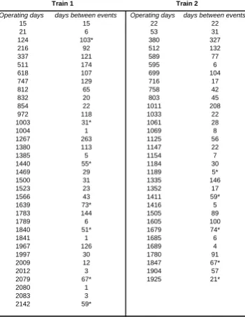
Table 1 presents the shutdown events reported for both trains based on the operating time (days). Shutdown data based on the operating time is preferred over the calendar time since the former represents the actual time the equipment is in operation. The analysis based on the operating time can show the actual condition of the system performance i.e. improving, deteriorating or unchanged [5] which may be unnoticeable if it is done on the calendar time. The operating time is defined as the calendar time minus the shutdown and standby time. The time between the events or also known as inter-arrival time is the time gap between two consecutive events. From the data, both trains experienced 27 failures during the observation period.
Table 1: Time of shutdown based on operation time (days)
Operating days days between events Operating days days between events
15 15 22 22
21 6 53 31
124 103* 380 327
216 92 512 132
337 121 589 77
511 174 595 6
618 107 699 104
747 129 716 17
812 65 758 42
832 20 803 45
854 22 1011 208
972 118 1033 22
1003 31* 1061 28
1004 1 1069 8
1267 263 1125 56
1380 113 1147 22
1385 5 1154 7
1440 55* 1184 30
1469 29 1189 5*
1500 31 1335 146
1523 23 1352 17
1566 43 1411 59*
1639 73* 1416 5
1783 144 1505 89
1789 6 1605 100
1840 51* 1679 74*
1841 1 1685 6
1967 126 1689 4
1997 30 1780 91
2009 12 1847 67*
2012 3 1904 57
2079 67* 1925 21*
2080 1
2083 3
2142 59*
Train 2 Train 1
* denotes PM events and end time observation
[image:2.595.306.482.527.754.2]B. Factors Influencing System Performance
After discussions with the plant personnel, the following factors or covariates are suspected to have influence on the system performance.
i. Train: Both trains are designed to produce similar performance, however based on the data, train 2 indicates longer shutdown duration than train 1. ii. Operation loading mode: When one train is down,
another train has to take up the entire load i.e. single loading. This extra loading may result in increased stress on that running train.
iii. Subsystem: Almost 50% of the failures come from gas turbine and gas compressor. It is useful to understand the impact of these failures to the overall system failure frequency.
iv. Start up operation: Frequent start up operation due to switching back of operation mode from shutdown or standby to operating could be detrimental since it can induce stresses on the equipment that lead to wear-out problem. The number of switching operation depends on the frequency of failures and standby mode events. In the case of standby mode, a start up operation is assumed only when the equipment has been in standby for more than four hours.
v. Maintenance activities: PM activities are supposed to reduce number of failures and increase the time between failures of the system. Sometimes the maintenance impact can be insignificant or detrimental to the system performance.
IV. METHODOLOGY
The analysis of the data is divided into two stages. The first stage is to look at the pattern of failures occurring over time for any possible trend indicating the non-steady state of the system performance i.e. improving or degrading. The next stage is to assess the impact of various factors or covariates on the system failure distribution as mentioned in the previous section, thus enable management to take appropriate actions if any of them is found to significantly deteriorate the system performance.
A. Trend Test
A trend plot of cumulative number of failures over time can provide a snapshot of how the system performance is heading to. When the inter-arrival time is getting shorter, the plot will tend to concave up implying that the system is deteriorating. The opposite condition is observed when the system is improving. A linear plot is an indicator that that the system performance is constant. Ascher and Feingold [7] refer these conditions as „sad‟, „happy‟ and „non-committal‟ system respectively. These system conditions can be assessed using an analytical trend test which basically tests whether the process has a monotonic trend or not (stationary). Ascher and Feingold [7] stress the important of trend test as the first step of the reliability data analysis and model development and this is strongly supported by other researchers [8-10]. Several trend tests had been developed, but the most commonly used
is the Laplace test. This test is used to statistically test for the null hypothesis that the failure distribution is stationary (HPP) against the alternative of a monotonic trend (NHPP). Other trend tests include MIL-HDBK-189 (HPP vs. non-HPP), Mann and Lewis-Robinson (renewable process, RP vs. a monotone trend) [7].
B. Laplace Trend Test
Consider the data consists of a series of n failures observed during the period of (0,tf). The Laplace test statistics, UL is
defined by
n t
t n
t
U
f f n
i i
L
12 1 2 1
1 (1)
where:
ti = the time to failure for ith event
n = total number of failures during the observation period (0, tf)
tf = observation end time (termination time). If the
observation end time is a failure time at nth event, the above expression need to be modified by replacing n with
n-1.
Under the null hypothesis, the test UL approximately follows
a standard normal distribution. Thus large positive or negative UL values suggest that the process is not stationary
(not HPP). The null hypothesis is rejected if UL is smaller than
a critical minimum value or greater than the maximum critical value read from the standard normal table for a given significance level. UL value greater than 0 indicates
degradation (concave up pattern) and less than 0 signifies improvement (concave down pattern) in the system performance.
C. Rate of Occurrence of Failure
The changes in the pattern of failures can also be detected by examining the failure rate trend against the time. For repairable system, the failure rate, or also known as the failure intensity, can be estimated by calculating the rate of occurrence of failure (ROCOF). For the HPP process, the graphical plot of ROCOF over time should be constant since the HPP process has a constant failure rate. ROCOF for interval i can be estimated by the mean failure rate, vi, which is
the number of failures occurred in the evenly distributed time interval (ti-ti-1) divided by that time interval;
1 1
i i
i i i
t t
t t
v numberoffailures in (2)
The graph shape of ROCOF is highly dependence on the selection of time interval, thus proper selection of the time interval is important. Smoothing technique such as kernel density smoothing can be used to smooth the graph [11].
D. Covariates Analysis
applications of PHM in repairable system are generally confined to the situation where the system failure distribution is assumed to behave like an HPP [13]. In the case of NHPP, the more appropriate model is the Proportional intensity models (PIM), an extension of the PHM. For detailed discussion on the PIM refer to [14,15]. The selection of which model to be used depends on the finding of trending test described earlier (HPP vs NHPP). Besides the PHM, a non-parametric Kaplan Meier (KM) estimator method can also be used as an exploratory tool. This method, however, is only suitable for univariate and not for multivariate analysis.
E. Modeling of covariates
Let the time to failures of n number of failures be t0, t1, t2,
t3,…,tn, with t0 < t1 < t2 < .. <tn. t0 is an arbitrary time which
mark the beginning of the observation period. The time between failures (inter-arrival) are denoted by Xi, where Xi = ti – ti-1. For an illustration, let consider a PM as the covariate
(Figure 2). Assume there is a PM activity being carried out in between t1 and t2. In this model the impact of that PM on the
failure distribution is measured basically by the length of X2;
how effective is the PM to extend the X2 period. All of the
covariates in this study follow the same notation except for the start up covariate, where the impact of start-up covariate is measured based on X3 instead of X2. Here, we are interested to
[image:4.595.305.545.237.304.2]know the impact of start up failures to the next failure event and not prior to that.
Fig. 2: Modeling of failures for PM covariate
V. DATA ANALYSIS AND RESULTS
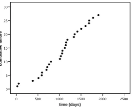
The trend plots of the cumulative number of failures over the operating time for both trains taken from Table 1 are shown in Figure 3 and 4 respectively.
2500 2000 1500 1000 500 0
time (days)
30
25
20
15
10
5
0
cum
ula
tiv
e
fai
lur
[image:4.595.304.548.328.399.2]e
Fig. 3: Cumulative failures versus operating days for Train 1
2500 2000 1500 1000 500 0
time (days)
30
25
20
15
10
5
0
cum
ula
tiv
e
fai
lur
e
Fig. 4: Cumulative failures versus operating days for Train 2
The trend plots for both trains exhibit a linear pattern an indication of the train performance is neither improving nor degrading. To test for this assumption, the statistical Laplace tests are conducted. For train 1, the calculated Laplace statistics value, UL is 1.66 and for train 2 is 0.68. These results were found not to be statistically significance at 95% confidence level (z = +/- 1.96). Thus the assumption based on the graphical method earlier is acceptable that the data do not exhibit any monotonic trend. This non-monotonic failure data trend suggests that the process can be modelled as an HPP. To look at how the failure rate change over time, ROCOF based on time interval of 200 days is calculated. The plots of ROCOF for respective train are shown in Figure 5 and 6. The plots have been smoothed using Gaussian kernel smoothing technique [16]with kernel bandwidth is set to 125 days.
0.00 0.02 0.04 0.06 0.08
0 200 400 600 800 1000 1200 1400 1600 1800 2000 2200
time (days)
fa
il
u
re
r
at
[image:4.595.43.287.377.442.2]e
Fig. 5: ROCOF against cumulative operating time for Train 1
0.00 0.02 0.04 0.06 0.08
0 200 400 600 800 1000 1200 1400 1600 1800 2000 2200
time (days)
fa
ilu
re
r
at
[image:4.595.52.193.521.627.2]e
Fig. 6: ROCOF against cumulative operating time for Train 2 The plots indicate that there are no increasing or decreasing trends in failure rates for both trains. The failure rate for train 1 looks rather constant with little fluctuation throughout the observation time. For train 2, the plot also exhibits somewhat constant trend over the time period. However, a slight increase in failure rate is noticeable near the midpoint of observation period. Based on the equation [2] the estimated failure rates for train 1 and 2 are around 0.013 and 0.014 respectively.
A. Analysis of Covariates
The next stage of analysis is to study whether the covariates are the critical factors affecting the system performance. Since the earlier testing indicates that the HPP is a suitable model for the system‟s failure distribution, the analysis on covariates can be done using Kaplan Meier estimator and PHM methods. In the following analyses the data for both trains are combined and analyzed assuming that both trains are having the same failure distribution.
B. Kaplan Meier Estimator
KM estimator [17] is a non-parametric method of estimating the reliability (survival) function from life-time data. It can be used for data with complete and censored events. The estimated reliability function, Ȓ(t), is a step function given by
t
t i
i
i n
d t
R() 1 (3)
Where Ȓ(t) is the estimated reliability for any particular point of time; ni is the number of individual at risk just prior to time,
ti ; and di is the number of individual that fails up during time
x1 x2 x3 … xn
t0 t1 PM t2 t3 … tn-1 tn
Failures
x1 x2 x3 … xn
t0 t1 t2 t3 … tn-1 tn Time
Failures
Observation period start
[image:4.595.53.191.655.766.2]period ti. Thus, Ȓ(t) is based on the conditional probability
that an individual survives at the end of interval provided that individual was existed at the start of the time period. Ȓ(t) is the product of these conditional probabilities and provides the point estimator for the reliability function at any particular time t.
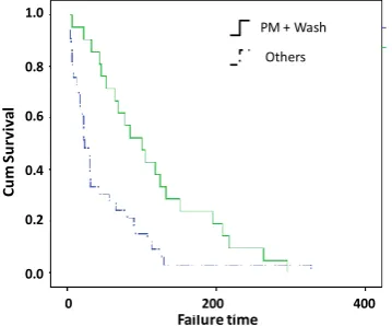
[image:5.595.53.288.337.430.2]The KM survival function plot can be used to visually compare the survival rates between two groups to determine which one is performing better (e.g. train 1 versus train 2). A statistical hypothesis test called the log-rank is employed to test the null hypothesis that there is no significant difference between the survival data of these two groups. Table 2 lists the grouping for each of the covariates. The covariates identified for the analysis were train, operation mode, sub-system, start up operation and maintenance activities. The maintenance activities, however, had been further broken down into two more covariates; the PM and PM plus engine wash. The PM covariate only includes 4K and 8K ppm but not engine wash. This will enable separate assessment to be done on the effectiveness of PM action with and without engine wash. The results of log-rank statistical tests calculated using SPSS software are tabulated in Table 3.
Table 2: Covariates and their grouping
Covariates Group 0 Group 1
Train Train 1 Train 2
Operation mode Shared load Single load
Subsystem Other sub-systems Gas Turbine + Compressor
Start-up operation Others Start-up failures
PM Others Failures after PM
PM + wash Others Failures after PM + engine wash
Table 3: Log-rank statistical test on covariates
covariates Train Operation Subsystem Start-up PM PM+Wash mode operation
chi sq. 0.046 0.027 3.34 0.01 2.41 8.52 sig. (P value) 0.83 0.087 0.07 0.9 0.12 0.004
The results indicate that only the PM plus wash covariate has significant effect on the system failure distribution (P-value less than 0.05). The results also show there is no significant difference between the two trains performance, thus the assumption that both trains have similar failure distribution is acceptable. Figure 7 describes the survival plot of PM plus wash covariate where it shows this covariate has a positive influence in extending the system inter-arrival failure time.
Failure time
0 0.6 0.8 1.0
200 400
0.0 0.2 0.4
C
u
m
Su
rv
iv
al
PM + Wash
[image:5.595.68.248.613.762.2]Others
Fig. 7: KM plot of cumulative survival for failures after PM plus engine wash vs. other failures
C. Proportional Hazards Model (PHM)
The PHM can be used to evaluate the simultaneouseffect of multiple covariates on the system failure distribution. Here, it enables the difference between the survival data of different groups to be tested while allowing for other covariates to be taken into consideration. The PHM or Cox regression model [18] is the most important distribution-free regression model used for the analysis of censored data [19]. In the PHM, the hazard function is composed of two parts; a baseline hazard function and a covariates dependent function. The model assumes a multiplicative effect of covariates to the baseline hazard function. The basic form of the PHM is given by
)
(
)
(
)
:
(
t
z
h
0t
z
h
T (4)Where ho(t) is the baseline hazard function, is the arbitrary
function of the row vector covariates, z, and is the column
vector of unknown regression parameters. can be represented in many functional forms, such as exponential, logistic and inverse linear and linear form. Cox [18] proposes an exponential function due to its simplicity. Thus the PHM with k covariates can be expressed as
) ... exp(
) ( ) :
(t z h0 t 1z1 2z2 kzk
h ()exp( )
1
0 i
k
i iz
t
h (5)
ho(t) is modeled as a non parametric thus making the PHM a
semi-parametric model.
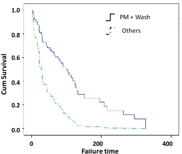
The results of PHM analysis on the covariates are shown in Table 4. Here, the results also indicate only PM plus wash is the influential factor with the statistical significant value (P value) is 0.044. This p-value is however higher than the one derived from the KM log-rank test (0.004) since the PHM model includes the effects of all covariates in the analysis. Based on the equation (5) the PHM plus wash covariate will reduce the hazard of failures for the system by a factor of 0.43. The estimated survival plot for PM plus wash covariate is shown in Figure 8.
Table 4: PHM results analysis on covariates
Covariates Std error Wald df Sig. (P value) Exp( )
Train .045 .296 .024 1 .878 1.046
Operation mode .533 .557 .917 1 .338 1.704
Subsystem -.368 .323 1.302 1 .254 .692
Start up operation .090 .405 .049 1 .824 1.094
PM .006 .466 .000 1 .989 1.006
PM + Engine
Failure time
0 0.6 0.8 1.0
200 400
0.0 0.2 0.4
C
u
m
Su
rv
iv
al
PM + Wash
[image:6.595.64.247.55.209.2]Others
Fig. 8: PHM plot of cumulative survival for failures after PM plus engine wash vs. other failures
VI. DISCUSSIONS ON RESULTS
The trend charts and Laplace test indicated both train 1 and 2 exhibited a linear and non-monotonic trend. The calculated ROCOF showed fairly similar results, where there were no indications of increasing failure rate trend in both trains. Train 2, however showed a slight ROCOF spike in the middle of the study period. The predicted failure rate for train 1 and 2 were 0.013 and 0.014 respectively, which was almost the same.
Covariates analysis using the PHM and KM techniques found that the train type is not an influencing factor determining the system failure events. There were no significant differences between both train failure performances. Nevertheless, in the aspect of downtime, based on the maintenance data train 2 had experienced downtime seven times higher than train 1. These downtime events had occurred mainly between 2003 and 2006.
The single operation mode was assumed to cause more failures due to increased in stress load on the individual train. Based on the number of failures occurred during this single mode operation, it was shown not a major factor. There were only four failures associated with this operation mode. Besides, the operation mode had been dominantly under shared mode since 2005 due to high production demand and decreased trend in failures with high downtime.
Failures associated with gas turbine and gas compressor were found not significantly difference compared to failures related to other subsystems. In term of downtime, however, both subsystems contribute to 60 and 90 percent of total downtime period for train 1 and train 2, respectively.
Based on the failures occur right after start up operation, the start up failure did not have any significant influence on the system failure distribution. The scope of the study, however, did not count the compounding effect of cumulative start up events due to limited data availability.
The analysis on maintenance activities revealed that the PM (4K and 8Kppm) did not have a significant influence on the system failure rates. Nevertheless, the PM together with engine wash was found to play a critical role in extending the inter-arrival time of failures thus improving the system performance.
VII. CONCLUSSIONS
In this paper, a systematic and effective approach of extracting and analyzing maintenance data to gain important
information about the system performance was clearly demonstrated. The approach was based on problem and data-driven rather than model and technique-led. The study found that the system failures is neither deteriorating nor improving and can be appropriately modeled by an HPP model. In analyzing the critical factors influencing the inter-arrival failure times, the non-parametric KM and PHM techniques were applied. These methods were shown to be adequate in identifying the critical factors affecting the system failure distribution.
ACKNOWLEDGMENT
The authors wish to thank Professor J. Ansell of University of Edinburgh for his valuable inputs and comments on the applications of various methods used in this study and the Universiti Teknologi PETRONAS for the financial support.
REFERENCES
[1] J. I. Ansell, and M. J. Phillips , Practical Methods for Reliability Data Analysis, Oxford University Press, 1994.
[2] T. Bendell, “An Overview of Collection, Analysis, and Application of Reliability Data in the Process Industries,” IEEE Transactions on Reliability, Vol. 37, No. 2, June 1988.
[3] R. Dekker, “Applications of maintenance optimization models: a review and analysis,” Reliability Engineering and System Safety, 51, 1996, p. 229-240.
[4] M. Modarres, M. Karminskiy, and V. Krivtsov, Reliability Engineering and Risk Analysis, Marcel Dekker, New York, 1999. [5] A. Hoyland, and M. Rausand, System Reliability Theory, Wiley,1994. [6] K. Muralidhan, “Review of repairable systems and point process
models”, ProbStat Forum, Volume 1, 2008.
[7] H. Ascher, and H. Feingold, Repairable Systems Reliability, Marcel Dekker, New York, 1984.
[8] B. H. Lindqvist, “On the Statistical Modeling and Analysis of Repairable Systems”, Statistical Science, Vol. 21, No. 4, 2006, p.532–551.
[9] T. Fu-rong, J. Zhi-bin, and B. Tong-shuo,“Reliability Analysis of Repairable Systems Using Stochastic Point Processes”, J. Shanghai Jiaotong Univ. (Sci.), 2008, 13(3): p. 366–369.
[10] D. M. Louit, R. Pascual, R. and A. K. S. Jardine,“A practical procedure for the selection of time to failure models based on the assessment of trends in maintenance data”, Reliability Engineering and System Safety, 2009.
[11] J. Ansell, et al, “Analysing maintenance data to gain insight into systems performance”, Journal of the Operational Research Society, 54, 2003, p. 343-349.
[12] M. Newby, “A critical look at some point-process models for repairable systems”, IMA Journal of Mathematics Applied in Business & Industry, Vol 4, 1993, p. 375-394.
[13] D. Kumar, “Proportional hazards modeling of repairable systems,”
Quality and Reliability Engineering International, vol 11, 1995, p. 361-369.
[14] D. Lugtigheid, D. Banjevic, and A. K. S. Jardine, “Modelling repairable system reliability with explanatory variables and repair and maintenance actions”, IMA Journal of Management Mathematics, 15, 2004, p. 89–110.
[15] S. T. Jiang, T. L. Landers, and T. R. Rhoads,“Assessment of Repairable-System Reliability Using Proportional Intensity Models: A Review”, IEEE Transactions on Reliability, Vol. 55, no. 2, June 2006. [16] K. Teknomo, (2007) Kernel Regression [Online]. Available:
http://people.revoledu.com/kardi/tutorial/regression/kernelregression/ [17] E. L. Kaplan, and P. Meier, “Nonparametric estimation from
incomplete observations”. Journal of the American Statistical Association, 53, 1958, p. 457-48.
[18] D. R. Cox, “Regression Models and Life Tables,” Journal of the Royal Statistical Society Series B, 34 (2): p.187–220, 1972.