An Assignment Model in Optimizing Wire Bond Total Utilization in Multiple Tool Type and Product Mix Environment

Abstract—“Efficiency” has been the key word for Intel last 2006 with focus of improving Total Utilization (TU) of tools in ATM. Total Utilization (TU) gives a clearer understanding of how much our capital is truly being used. In order for us to realize a higher total utilization, we need to ensure that our tools are productive majority of the time.

In Chipsets assembly, Wire Bond is considered the constraint tool of the production floor. Cavite Chipsets assembly has the largest fleet of wire bonders across virtual factories and contributes to 20% of the total Intel Chipsets assembly output. Furthermore, internal assembly cost is cheaper compared to external assembly. Thus, it is critical that this station is maximized and ensure that it is meeting POR (Plan of Record) goals.

However, in WW 01’06 to WW 26’06, Wire Bond Total Utilization (TU) Performance is struggling to meet POR (Plan of Records) utilization of 81% and only averaging 68%. There is a need to get Wire Bond tool performance on track to meet the Goal Utilization (GU) as soon as possible to prevent additional cost to Intel operations.

In this paper, the author will discuss the method used in identifying the root cause of the problem. The author will also demonstrate how an assignment model can be an alternative solution in optimizing Wire Bond Total Utilization leading to an improved idle time from 35 hours to 9 hours per week.

Index Terms— Efficiency, Total Utilization, Idle Time, Wire Bond

I. INTRODUCTION

Highlight Total Utilization (TU) is one of the key indicators in Intel’s efficiency drive across ATM. ATM IE (2006) defines Total Utilization as the percent of productive time during total time where

in total time is equivalent to 168 hours always. There are two (2) ways to calculate Total Utilization in ATM; the “time-based” and the “outs-based”.

Equation (1) and (2) shows the formula for calculating Total Utilization using “time-based” and “outs-based” approach. “Time-based” calculation is normally used for stations with AEPT while the “outs-based” calculation is used for non-AEPT enabled tools.

Manuscript received October 9, 2007. This work was supported by Intel Technology Philippines, Inc.

A.Y. Fong is with the Industrial Engineering Department , Intel Technology, Cavite, Philippines (phone: +639209381579; email:

Time-based:

∑

Inventory Tool

me oductiveTi n

Utilizatio

Total_ (Pr /168)*100/ _ (1)

Outs-based:

inventory tool yield stage rate machine

outs stage n

Utilizatio Total

product

i i i

i

_ 100 * _ * _ * 168

_

_ _⎟⎟

⎠ ⎞ ⎜

⎜ ⎝ ⎛

⎟⎟ ⎠ ⎞ ⎜⎜

⎝ ⎛ = ∑

(2) The two (2) equations, at first glance, look different. However, closer inspection of the formula will yield the same result that is productive time over total time, which is equivalent to Total Utilization (TU). For Wire Bond, we will use equation (2) to calculate for Total Utilization (TU) since this is a non-AEPT station.

The succeeding sections will discuss the Total Utilization Concept further, the problem, the root cause, hypothesis and solution which will lead to the successful recovery of Wire Bond in its Actual Utilization (AU) performance back to 81%.

II. THE TOTAL UTILIZATION CONCEPT

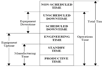
In the introduction, we present the equations used in ATM to calculate for Total Utilization (TU). In this section, we will take it a step further and understand the concept of Total Utilization (TU) by looking at the equipment states that is included in the Total Time per week (168 hours). Figure 1 shows the equipment states stack chart into which all equipment conditions must be classified.

Figure 1. Equipment States Stack Chart

There are six (6) basic equipment states to be considered in measuring tool performance. The equipment states and their

An Assignment Model in Optimizing Wire Bond

Total Utilization in Multiple Tool Type and

Product Mix Environment

respective definitions as stated in SEMI E10 (2004) are as follows [2]:

1. Productive Time - The time when the equipment is

performing its intended function.

2. Standby Time - The time when the equipment is in a

condition to perform its intended function, but is not operated.

3. Engineering Time - The time when the equipment is in a

condition to perform its intended function, but is operated to conduct engineering experiments.

4. Scheduled Downtime - The time when the equipment is

not available to perform its intended function due to planned downtime events.

5. Unscheduled Downtime - The time when the equipment

is not in a condition to perform its intended function due to unplanned downtime events.

6. Non-scheduled Downtime - Time when the equipment is

not scheduled to be utilized in production, such as unworked shifts, weekends, and holidays.

Total Utilization gives a clearer understanding of how much our capital is truly being used. In order for us to realize a higher total utilization, we need to ensure that our tools are productive majority of the time – that is increase productive time and minimize everything else.

III. THE PROBLEM AND ITS ROOT CAUSE

In Chipsets assembly operations, Wire Bond is the bottleneck station. The output of these tools contributes to 20% of the total Intel ICH assembly output. Furthermore, for each unit produced internally, a cost savings is realized.

From WW 01’06 to WW 26’06, it was observed that Wire Bond Total Utilization (TU) is struggling to meet the 81% goal with an average of 68% only as shown in Historical data illustrated in Figure 2. Thus, there is a need to get Wire Bond on track to meet the 81% Goal Utilization (GU).

Figure 2. Wire Bond Overall Total Utilization Performance (WW01’06 to WW 26’06)

Data collected by Engineering from WW 01’06 to WW 26’06 reveals that 60% of the total downtime of the tools is driven by idle time. Figure 3 pie chart shows the breakdown

of downtime between scheduled downtime, unscheduled downtime and standby time.

Figure 3. Total Downtime Breakdown

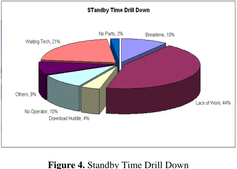
Further drilling down the standby time in Figure 4 using the same data source reveals that 44% of the standby time is caused by lack of work. Another 40% is due to waiting for MS due to break time, no operator and waiting for technicians. The remaining 16% is due to huddles/download, no parts and others.

Figure 4. Standby Time Drill Down

A. Root Cause Analysis and Interpretation

Figure 5. Pareto Chart for Causes of Standby Time

Following the 80-20 rule, standby time can be solved by minimizing lack of work, waiting for Technician, and waiting for MS due to break time and no operator. To further simplify, we can refer to waiting for Technician and MS as inefficient headcount resource management. Solving these root causes will help Wire Bond meet the 81% Goal Utilization (GU).

B. Further Investigation on Lack of Work and Inefficient Headcount Resource Management

From previous section, we narrowed down the root cause of standby time and focused on lack of work and inefficient headcount resource management. In this section, we will try to understand further why lack of work and inefficient headcount resource management became top contributor of standby time.

Data showed in previous section revealed that lack of work makes up 44% of the total standby time of Wire Bond. There are three (3) known possible reasons for lack of work. 1. Volume loading is low which results in capacity not being

fully utilized.

2. Excess tool inventory in the production floor.

3. Suboptimal allocation of equipment resources between products and equipment models.

Among the three (3) possible reasons for lack of work, we can easily disregard excess tool inventory for Wire Bond since there is none. Chipsets assembly is ideally maximized since it is cheaper than external alternative. This leaves us to investigate further if the internal assembly loading and how equipment resources are allocated between products and equipment models is the main causes of lack of work for Wire Bond.

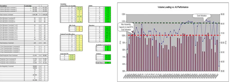
Figure 6 shows the comparison between the weekly assembly volume loading and actual utilization (AU) performance of Wire Bond from WW 01’06 to WW 26’06.

Figure 6. Volume Loading vs. Actual Utilization (AU) Performance (WW 01’06 to WW 26’06)

A closer inspection of figure 6 confirms that internal capacity of Wire Bond is not fully utilized. On the average, actual internal volume loading for Wire Bond is at 90%/wk versus the maximum internal capacity. However, it is also important to note that on weeks wherein the loading is greater than or equal to 100%/wk the 81% goal utilization (GU) was still unachievable. This instance can be further explained in Figure 7.

Figure 7. Comparison of Actual Utilization (AU) between Machine A, B and C

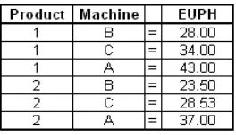
Figure 7 shows the actual utilization (AU) per bonder type. It is evident from the figure that imbalances in the way we utilize our bonders exist. Analyzing the data reveals that we are prioritizing machine A over machine B and C model in producing units – that is more units moved-in in Machine A compared to the other bonder type. This can cause problem in Total Utilization (TU) of our bonders. Figure 8 shows the comparison of EUPH of each bonder type per product.

Just by looking at the EUPH of machines A, B and C in Figure 8, one (1) machine A is equivalent to 1.5 machine B bonder and 1.3 machine C bonder. Mathematically, loading one (1) machine A will result in 1.5 machine B and 1.3 machine C bonders idle in a week. This will result in drop of TU since overall productive time of your bonders will be low because of the idling machine B and C bonders making this decision suboptimal. An optimal loading between Machine A, B and C must be achieved even at full capacity in order to realize the 81% Goal Utilization (GU).

As for the inefficient headcount resource management, data shows it contributes 40% to the total standby time of Wire Bond. 20% of this is caused by waiting for Technician and the other 20% is caused by waiting for MS due to break time and no operator. Between waiting for Technician and waiting for MS, waiting for technician can be considered as unavoidable standby time since there are only 10 technicians in a shift covering hundreds of machines. With this ratio of technician versus Wire Bond, there is a possibility that some tools will be waiting before a technician can do the repair. On the other hand, waiting for MS can be considered avoidable standby time especially during break times since measures can be taken to prevent this. One way is to ensure that enough certified headcount is available to cover Wire Bond during break time as flex headcount. A 20% standby time due to break time and no operator indicates that this is not happening across all bonders.

C. Synthesis of the Problem

Further analysis of data in the previous sections revealed that there are three (3) underlying root causes for the high standby time in Wire Bond: (1) Inability to maximize capacity; (2) Suboptimal allocation of equipment resources between products and equipment models; (3) Lack of certified headcount to cover during breaks and absences contributing to equipment idling.

Among these three (3) root causes, the most important to address is the maximization of capacity. However, it has been proven that as long as suboptimal loading exist between machine A, B, and C, 81% Goal Utilization (GU) cannot be achieved even at maximum capacity. In the next chapter, the author will discuss the assignment model formulated to optimize machine A, B and C.

IV. IMPROVEMENT PHASE

Assignment models are actually a special case of the transportation model in which the workers represent the sources and the jobs represent the destinations [4]. The objective of assignment models is to find “the best person for the job” [4]. Assignment models can also be applied in assigning machines, or vehicles, or plants, or even time slots with consideration to capability or skill of the assignee [1]. As an example, Smith (2004) wrote a thesis about a Robust Airline Fleet Assignment based on Fleet Assignment Model developed by Hane (1995) which aims to maximize operating profit while ensuring balance in assignment of fleet type, flow in the timeline of aircraft and ensure that total aircraft assigned won’t exceed inventory [3].

To optimize loading between machine A, B and C and achieve the goal utilization (GU) of 81% in Wire Bond, an assignment model will also be formulated. The author chose to formulate an assignment model to solve the problem since we want to know how many units of product i will bonder j produce to maximize Total Utilization (TU) of Wire Bond.

A. The Assignment Model to Maximize Wire Bond Total Utilization (TU)

In this section, we describe the assignment model for Wire Bond. We start of by defining the set and decision variables to be used in the model with corresponding notation. Set:

i – refers to the bonder type j – refers to the product

EUPH ij - refers to the EUPH of bonder i processing product j

RR ij - refers to the Runrate of bonder i processing product j V j – refers to the volume per product

T i – refers to the inventory per bonder type Decision Variable

i – refers to the bonder type j – refers to the product

M ij – refers to the move-in quantity in bonder i of product j Now that the set and decision variables has been defined, we now proceed with formulating the model itself. Equation (3) below defines the objective function of the model. As stated below, the overall objective of the model is to maximize Total Utilization (TU).

INV xEUPHij Mij

TU Max

tool

i product

j

/ ))] 168

/( ( [

_ =

∑ ∑

(3)

Afterthe objective function, the constraints will now be defined. Equation (4) below is the Volume Allocation Constraint. This ensures that the total move-in quantity will not exceed the volume set to be loaded for the week per product.

∑

∑

j tool

i

Vj

Mij (4)

Equation (5) below defines the Tool Allocation Constraint. This ensures that the total tools allocated to produce a certain move-in quantity of product will not exceed tool inventory per bonder type.

∑

∑

j tool

i

Ti RRij Mij/ )

( (5)

∑

∑

∑

j

tool

i tool

i

Ti RRij

Mij/ )

( (6)

Equation (7) defines the Tool Characterization Constraint. This ensures that the model will return a value of 0 in the Move-in quantity for a bonder type if it is not qualified to run a certain product.

0

=

Mij (7)

Equation (8) defines the Total Productive Time Constraint. This ensures that total productive time for all bonders will not exceed 168 hours multiplied to total tool inventory.

∑

∑

∑

j

tool

i tool

i

Ti x EUPHij

Mij/ ) (168 )

( (8)

Equation (9) defines the Productive Time Constraint per Bonder Type. This ensures that productive time per bonder type will not exceed 168 hours multiplied to tool inventory per bonder type.

∑

∑

j tool

i

xTi EUPHij

Mij/ ) (168 )

( (9)

Lastly, Equation (10) defines the Non-negativity Constraint. This ensures that the model will not return a negative value for move-in quantity. A negative value solution will automatically indicate infeasible.

0

>=

Mij (10)

V. IMPLEMENTATION PHASE AND RESULTS

In the previous section, the assignment model was presented in a mathematical equation. The equations are then transferred to Microsoft Excel after making sure everything is considered in the assignment model. It is called the TU Calculator following its primary purpose. Figure 9 shows TU Calculator in Excel.

Figure 9. TU Calculator in Excel

Using Excel Solver, TU calculator computes for the optimal loading of machine A, B and C to be able to maximize Total Utilization (TU). Using WW 04’06 and 09’06 volume loading of assembly which is greater than or equal to 100%/wk, we test the model and compare to the actual results on the said work weeks. Table 1 shows the comparison between the TU calculator and actual results on WW 04’06 and 09’06.

Table 1. Comparison Between TU Calculator and Actual Results WW04’06 and WW09’06

Results found in Table 1 confirm the claim that even at 100%/wk loading, there is still a need to optimize loading between machine A, B and C to yield a higher Total Utilization (TU). Also, it confirms that prioritizing Machine A will yield a lower Total Utilization (TU) since it idle more machine B and C Wire Bonders. Thus, assignment model can be used to improve Total Utilization (TU) of tools.

With this result, TU calculator has been used starting WW 27’06 to guide manufacturing in terms of Wire Bond Total Utilization (TU) improvement efforts. Every week, IE releases an email update on the Total Utilization (TU) performance for the previous week and provide forecast TU for next week based on the TU Calculator results. Also, learning sessions with Supervisors were conducted in the production floor to explain further the impact of loading too much to machine A versus B and C Wire Bond. They are also encouraged to address the problem of inefficient headcount management to support Wire Bond during break time and absences.

Figure 10 shows the improvement in the Actual Utilization (AU) of Wire Bond after solutions have been implemented from 68% on the average to a peak of 83%.

Aside from this, Total Standby Time for Wire Bond improved significantly from 35 hours/week to 9 hours/week. Figure 11 shows the Total Standby Time Trend from WW 01’06 to WW 52’06. You will observe a big improvement in Standby Time starting WW 27.

Figure 11. Wire Bond Standby Time Performance WW01’06 to WW 52’06

Also, standard deviation of machine A, B and C bonders improved from 5.15% to 4.68% making the operation more stable. See Figure 12.

Figure 12. Standard Deviation Plot for 8020, 8028 and Maxum+ TU Performance WW01’06 to WW 52’06

On top of this, the improvement enabled Intel to save $90,000 per week due to improved utilization of Wire Bonders.

VI. CONCLUSION AND RECOMMENDATION

In this paper, the author discussed the concept of Total Utilization (TU) and the problem in Wire Bond. Details as to why Wire Bond cannot meet the 81% Goal Utilization (GU) were reviewed and discovered that lack of work and inefficient headcount management is contributing to 60% standby time in Wire Bond. An interesting scenario where in Wire Bond is loaded more than max capacity of 100%/wk but still it cannot meet the Goal Utilization (GU) of 81% was investigated. It was hypothesized that Goal Utilization (GU) of 81% cannot be met even at maximum capacity because of suboptimal loading between machine A, B and C.

Assignment model formulated was used to prove that indeed suboptimal loading between machine A, B and C is causing lower Total Utilization (TU) for Wire Bond. The use of assignment model to solve suboptimal loading between machine A, B and C is justified since there are also other works with similar purpose like Hane (1995) and Smith (2004) though it was intended to be used for another industry. Aside from this, authors such as Hillier and Lieberman (1995) and Taha (2003) supported that the objective of assignment models is to find “the best person for the job”.

In the end, total standby time per week of bonders was reduced from 35 hours to 9 hours per week. Actual Utilization (AU) performance improved from average 68% to a peak of 83% per week. Standard deviation across machines A, B and C Total utilization Performance improved by 1%. Thus, it saved Intel $90,000 per week due to improved utilization of Wire Bonders.

In conclusion, using Assignment models can be an alternative approach to improving Total Utilization aside from bagging tools which is a normal practice in ATM to increase TU. This is particularly helpful when we see imbalances in the way we allocate resources to run products.

ACKNOWLEDGEMENTS

• Rey Villaflor, Romel Calpo, Eric Tamondong, Jojo Puenteblanca, Shierley Oraiz and Melita Lagdan for excellent manufacturing execution by ensuring all resources to support Wire Bond are available and plans to improve Total Utilization (TU) performance is being executed.

• Diana Biel for helping gather and share engineering data and continuously working on improving Wire Bond downtime.

• William Cantor for enabling automation tools that help track tool performance real time in the production floor.

• Cristina Fernandez and Emilio De Villa for fixing the ATM to Subcon rigid loading guidelines that helped maximize internal assembly capacity.

REFERENCES

[1] F. Hillier, G. Lieberman, “Introduction to Operations Research 6th Edition,” McGraw-Hill, Singapore, 2001, p 329.

[2] SEMI (2004). “Specification for Definition and Measurement of Equipment Reliability, Availability and Maintainability (RAM).,” available on-line, www.semi.org.

[3] B. Smith, “Robust Airline Fleet Assignment.” PhD Dissertation, Georgia Institute of Technology, 2004.

[4] H. Taha, “Operations Research: An Introduction 6th

Edition,” Prentice-Hall, Singapore, 2003, p 194-198.

Intel®

is a registered trademark of Intel Corporation or its subsidiaries in the United States and other countries.