Text Segmentation Using Exponential Models

(1)

Text Segmentation Using Exponential Models*

Doug Beeferman

Adam Berger

John Lafferty

S c h o o l o f C o m p u t e r S c i e n c e C a r n e g i e M e l l o n U n i v e r s i t y

A b s t r a c t

This paper introduces a new statistical approach to partitioning text automatically into coherent segments. Our approach en- lists both short-range and long-range language models to help it sniff out likely sites of topic changes in text. To aid its search, the system consults a set of simple lexical hints it has learned to associate with the presence of boundaries through inspection of a large corpus of annotated data. We also propose a new probabilistically motivated error metric for use by the natural language processing and information retrieval communities, intended to supersede precision and recall for appraising segmentation algorithms. Qualitative assessment of our algorithm as well as evaluation using this new metric demonstrate the effectiveness of our approach in two very different domains, Wall Street Journal articles and the T D T Corpus, a collection of newswire articles and broadcast news transcripts.

1 I n t r o d u c t i o n

The task we address in this paper might seem on the face of it rather elementary: identify where one region of text ends and another begins. This work was motivated by the observations that such a seemingly simple problem can actually prove quite difficult to automate, and t h a t a tool for partitioning a stream of undifferentiated text (or multimedia) into coherent regions would be of great benefit to a number of existing applications.

The task itself is ill-defined: what exactly is meant by a "region" of text? We confront this issue by

*Research supported in part by NSF grant IRI- 9314969, DARPA AASERT award DAAH04-95-1-0475, and the ATR Interpreting Telecommunications Research Laboratories.

adopting an empirical definition of segment. At our disposal is a collection of online d a t a (38 million words of Wall Street Journal archives and another 150 million words from selected news broadcasts) annotated with the boundaries between regions-- articles or news reports, respectively. Given this input, the task of constructing a segmenter m a y be cast as a problem in machine learning: glean from the d a t a a set of hints about where boundaries occur, and use these hints to inform a decision on where to place breaks in unsegmented data.

A general-purpose tool for partitioning expository text or multimedia d a t a into coherent regions would have a number of immediate practical uses. In fact, this research was inspired by a problem in information retrieval: given a large unpartitioned collection of expository text and a user's query, return a collection of coherent segments matching the query. Lack- ing a segmenting tool, an II:t application m a y be able to locate positions in its database which are strong matches with the user's query, but be unable to de- termine how much of the surrounding d a t a to provide to the user. This can manifest itself in quite unfortunate ways. For example, a video-on-demand application (such as the one described in (Christel et al., 1995)) responding to a query about a recent news event may provide the user with a news clip related to the event, followed or preceded by part of an unrelated story or even a commercial.

Document summarization is another fertile area for an automatic segmenter. Summarization tools often work by breaking the input into "topics" and then summarizing each topic independently. A segmentation tool has obvious applications to the first of these tasks.

The output of a segmenter could also serve as input to various language-modeling tools. For instance, one could envision segmenting a corpus, clas- sifying the segments by topic, and then constructing topic-dependent language models from the gen- erated classes.

(2)

very briefly review some previous approaches to the text segmentation problem. In Section 3 we describe our model, including the type of linguistic clues it looks for in deciding when placing a partition is ap- propriate. In Section 4 we describe a feature induction algorithm that automatically constructs a set of the most informative clues. Section 5 shows exam- ples of the feature induction algorithm in action. In Section 6 we introduce a new, probabilistically motivated way to evaluate a text segmenter. Finally, in Section 7 we demonstrate our model's effectiveness on two distinct domains.

2 S o m e P r e v i o u s Work

In this section we very briefly discuss some previous approaches to the text segmentation problem.

2.1 T e x t t i l i n g

The Te~ctTiling algorithm, introduced by Hearst (Hearst, 1994), segments expository texts into multiple paragraphs of coherent discourse units. A co- sine measure is used to gauge the similarity between constant-size blocks of morphologically analyzed to- kens. First-order rates of change of this measure are then calculated to decide the placement of boundaries between blocks, which are then adjusted to co- incide with the paragraph segmentation, provided as input to the algorithm. This approach leverages the observation that text segments are dense with repeated content words. Relying on this fact, however, may limit precision because the repetition of concepts within a document is more subtle than can be recognized by only a "bag of words" tokenizer and morphological filter.

Word pairs other than "self-triggers," for example, can be discovered automatically from training data using the techniques of mutual information employed by our language model. Furthermore, Hearst's approach segments at the paragraph level, which may be too coarse for applications like information retrieval on transcribed or automatically recognized spoken documents, in which paragraph boundaries are not known.

2.2 Lexical c o h e s i o n

(Kozima, 1993) employs a "lexical cohesion profile" to keep track of the semantic cohesiveness of words in a text within a fixed-length window. In con- trast to Hearst's focus on strict repetition, Kozima uses a semantic network to provide knowledge about related word pairs. Lexical cohesiveness between two words is calculated in the network by "acti- vating" the node for one word and observing the "activity value" at the other word after some number of iterations of "spreading activation" between nodes. The network is trained automatically using a

language-specific knowledge source (a dictionary of definitions). Kozima generalizes lexical cohesiveness to apply to a window of text, and plots the cohesiveness of successive text windows in a document, identifying the valleys in the measure as segment boundaries.

A graphically motivated segmentation technique called dotplotting is offered in (Reynar, 1994). This technique uses a simplified notion of lexical cohesion, depending exclusively on word repetition to find tight regions of topic similarity.

2.3 Decision t r e e s

(Litman and Passonneau, 1995) presents an algorithm that uses decision trees to combine multiple linguistic features extracted from corpora of spoken text, including prosodic and lexical cues. The decision tree algorithm, like ours, chooses from a space of candidate features, some of which are similar to our vocabulary questions. The set of candidate questions in Litman and Passonneu's approach, however, is lacking in features related to "lexical cohesion." In our work we incorporate such features by using a pair of language models, as described below.

3 A F e a t u r e - B a s e d A p p r o a c h

Our attack on the segmentation problem is based on a statistical framework that we call feature induction for random fields and exponential models (Berger, Della Pietra, and Della Pietra, 1996; Della Pietra, Della Pietra, and Lafferty, 1997). The idea is to construct a model which assigns to each position in the data stream a probability that a boundary be- longs at that position. This probability distribution arises by incrementally building a log-linear model that weighs different "features" of the data. For sim- plicity, we assume that the features are binary questions.

To illustrate (and to show that our approach is in no way restricted to text), consider the task of partitioning a stream of multimedia data containing audio, text and video. In this setting, the features might include questions such as:

• Does the phrase COMING UP appear in the last ut- terance of the decoded speech?

• Is there a sharp change in the video stream in the last 20 frames?

• Does the language model degrade in performance in the next two utterances?

• Is there a "match" between the spectrum of the current image and an image near the last segment boundary?

• Are there blank video frames nearby?

(3)

The idea of using features is a natural one, and indeed other recent work on segmentation, such as (Litman and Passonneau, 1995), adopts this approach. We take a unique approach to incorporat- ing the information inherent in various features, using the statistical framework of exponential models to choose the best features and combine them in a principled manner.

3.1 A s h o r t - r a n g e m o d e l o f l a n g u a g e

Central to our approach to segmenting is a pair of tools: a short- and long-range model of language. Monitoring the relative behavior of these two models goes a long way towards helping our segmenter sniff out natural breaks in the text. In this section and the next, we describe these language models and explain their utility in identifying segments.

The trigram models Ptri(W ]w-2, W-l) we em- ploy use the Katz backoff scheme (Katz, 19877) for smoothing. We trained trigram models on two different corpora. The Wall Street Journal corpus ( W S J ) is a 38-million word corpus of articles from the news- paper. The model was constructed using a set },V of the approximately 20,000 most frequently occurring words in the corpus. Another model was constructed on the Broadcast News corpus (BN), made up of approximately 150 million words (four and a half years) of transcripts of various news broadcasts, including CNN news, political roundtables, N P R broadcasts, and interviews.

By restricting the conditioning information to the previous two words, the trigram model is making the simplifying assumption--clearly false--that the use of language one finds in television, radio, and news- paper can be modeled by a second-order Markov process. Although words prior to w-2 certainly bear on the identity of w, higher-order models are impracti- cal: the number of parameters in an n-gram model is O([ W ]~), and finding the resources to compute and store all these parameters becomes a hopeless task for n > 3. Usually the lexical myopia of the trigram model is a hindrance; however, we will see how a segmenter can in fact make positive use of this shortsightedness.

3.2 A l o n g - r a n g e m o d e l o f l a n g u a g e

One of the fundamental characteristics of language, viewed as a stochastic process, is that it is highly

nonstationary.

Throughout a written document and during the course of spoken'conversation, the topic evolves, affecting local statistics on word oc- currences. A model which could adapt to its recent context would seem to offer much over a stationary model such as the trigram model. For example, an adaptive model might, for some period of time after seeing a word like HOMERUN, boost the probabilities

of the words {HOMERUN, PITCHER, FIELDER, ER- ROR, BATTER, TRIPLE, OUT}. For an empirically- driven example, we provide an excerpt from the B N corpus. Emphasized words mark where a long- range language model might reasonably be expected to outperform (assign higher probabilities than) a short-range model:

Some doctors are more s k i l l e d at doing the p r o c e d u r e than others so it's r e c o m - m e n d e d that p a t i e n t s ask d o c t o r s about their track record. People at high r i s k of s t r o k e include those over age 55 with a family h i s t o r y or high b l o o d p r e s s u r e , d i a b e t e s and smokers. We urge them to be evaluated by their family physicians and this can be done by a very simple p r o - c e d u r e simply by having them t e s t with a s t e t h o s c o p e for s y m p t o m s of blockage. One means of injecting long-range awareness into a language model is by retaining a cache of the most recently seen n-grams which is smoothed together (typically by linear interpolation) with the static model; see for example (Jelinek et al., 1991; Kuhn and de Mori, 1990). Another approach, using maximum entropy methods, introduces a parameter for

trigger pairs

of mutually informative words, so that the occurrence of certain words in recent context boosts the probability of the words that they trigger (Lau, Rosenfeld, and Roukos, 1993).

The method we use here, described in (Beefer- man, Berger, and Lafferty, 1997), employs a static trigram model as a "prior," or default distribution, and adds certain features to a family of conditional exponential models to capture some of the nonstationary features of text. The features are simple trigger pairs of words chosen on the basis of mutual information. Figure 1 provides a small sample of the

(s,t)

trigger pairs used in most of the experiments we will describe.

To incorporate triggers into a long-range language model, we begin by constructing a standard, static backoff trigram model Ptri (w ] w_ 2, w_ 1 ) as described in 3.1. We then build a family of conditional exponential models of the general form

pexp(W I H) =

Z(H)

exp

Aifi(H,w)

Ptri(W I w-2, w-1)

where

H ~ W-N,W-N+l,...,w-x

is the word

his-

tory

(the N words preceding w in the text), and

Z(H)

is the normalization constant

Z(H) =

(4)

($, t) e A RESIDUES, CARCINOGENS 2.3 CHARLESTON, SHIPYARDS 4.0 MICROSCOPIC, CUTICLE 4.1

DEFENSE, DEFENSE 8.4

TAX, TAX 10.5

KURDS, ANKARA 14.8

VLADIMIR, GENNADY 19.6

STEVE, STEVE 20.7

EDUCATION, EDUCATION 22.2

MUSIC, MUSIC 22.4

INSURANCE, INSURANCE 23.0

PULITZER, PRIZEWINNING 23.6

YELTSIN, YELTSIN 23.7

RUSSIAN, RUSSIAN 26. I

SAUCE, T E A S P O O N 27.1

FLOWER, PETALS 32.3

CASINOS, HARRAH'S 42.8

DRUG, DRUG 47.7

CLAIRE, CLAIRE 80.9

PICKET, SCAB 103.1

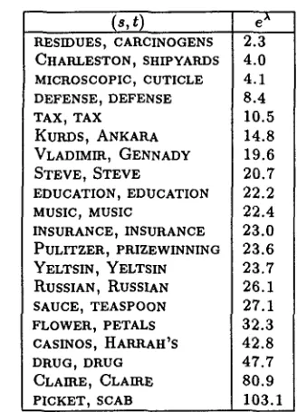
Table 1: A sample of the 84,694 word pairs from the B N domain. Roughly speaking, after seeing an "s" word, the empirical probability of witnessing the corresponding "t" in the next N words is boosted by the factor in the third column. In the experiments described herein, N = 500. A separate set of (s, t) pairs were extracted from the W S J corpus.

The functions fi, which depend both on the word history H and the word being predicted, are the features; each

fl

is assigned a weight A£. In the models that we built, feature

fi

is an indicator function, testing for the occurrence of a trigger pair

(si,tl):

1 i f s i E H a n d w = t i

fi(H,w)=

0

otherwise.

The above equations reveal t h a t the probability of a word t involves a sum over all words s such that s E H (s appeared in the past 500 words) and (s, t) is a trigger pair. One propitious manner of view- ing this model is to imagine that, when assigning probability to a word w following a history of words

H,

the model "consults" a cache of words which appeared in H and which are the left half of some (s, t) trigger pair. In general, the cache consists of content words s which promote the probability of their mate

t,

and correspondingly demote the probability of other words. As described in (Beeferman, Berger, and Lafferty, 1997), for each

(s,t)

trigger pair there corresponds a real-valued parameter A; the probability of t is boosted by a factor of e x for W words following the occurrence of si.

The training algorithm we use for estimating the A values is the

Improved Iterative Scaling

algorithm of (Della Pietra, Della Pietra, and Lafferty, 1997),

which is a scheme for solving the m a x i m u m likelihood problem that is "dual" to a corresponding maximum entropy problem. Assuming robust esti- mates for the A parameters, the resulting model is essentially guaranteed to be superior to the trigram model.

For a concrete example, if si-~-VLADIMIR and

ti

=GENNADY,

then fi = 1 if and only if VLADIMIR appeared in the past N words and the current word w is GENNADY. Consulting Table 1, we see t h a t in the B N corpus, the presence of VLADIMIR will boost the probability of GENNADY by a factor of 19.6 for the next N = 500 words.

3.3 L a n g u a g e m o d e l "relevance" features

A long-range language model such as that described in Section 3.2 uses selected words from the past ten, twenty or more sentences to inform its decision on the possible identity of the next word. This is likely to help if all of these sentences are in the same document as the current word, for in that case the model has presumably begun to adapt to the idiosyncra- cies of the current document. In the case of the trigger model described above, the cache will be filled with "relevant" words. In this setting, one would expect a long-range model to outperform a trigram (or other short-range) model, which doesn't avail itself of long-range information.

O n the other hand, if the present document has just recently begun, the long-range model is wrongly conditioning its decision on information from a different--and presumably unrelated--document. A soap commercial, for instance, doesn't benefit a long-range model in assigning probabilities to the words in the news segment following the commercial. Often a long-range model will actually be misled by such irrelevant context; in this case, the myopia of the trigram model is actually helpful.

By monitoring the long- and short-range models, one might be more inclined towards a partition when the long-range model suddenly shows a dip in performance--a lower assigned probability to the observed words--compared to the short-range model. Conversely, when the long-range model is consistently assigning higher probabilities to the observed words, a partition is less likely.

This motivates a quantitative measure of "relevance," which we define as the logarithm of the ratio of the probability the exponential model assigns to the next word (or sentence) to that assigned by the short-range trigram model:

a(H,w)=-log(

Pexp(wlH)

~kPtri(W I W - 2 W - 1 ) J "

[image:4.612.104.268.70.297.2]

(5)

If we observe the behavior of R as a function of the position of the word within a segment, we find t h a t on average R slowly increases from below zero to well above zero. Figure 1 gives a striking graphi- cal illustration of this phenomenon. T h e figure plots the average value of R as a function of relative position in the segment, with position zero indicating the beginning of a segment. This plot shows t h a t when a segment b o u n d a r y is crossed the predictions of the adaptive model undergo a d r a m a t i c and sud- den degradation, and then steadily become more ac- curate as relevant content words for the new segment are encountered and added to the cache. (The few very high points to the left of a segment b o u n d a r y are primarily a consequence of the word CNN--which is a trigger word and often appears at the beginning and end of a broadcast news segment.)

This observed behavior is consistent with our ear- lier intuition: the cache of the long-range model is destructive early in a document, when the new content words bear little in c o m m o n with the content words f r o m the previous article. Gradually, as the cache fills with words drawn from the current article, the long-range model gains s t e a m and R improves. While Figure 1 shows t h a t this behavior is very pro- nounced as a "law of large numbers," our feature induction results indicate t h a t relevance is also a very good predictor of boundaries for individual events.

In the experiments we report in this paper, we assume t h a t sentence boundaries are provided in the annotation, and so the questions we ask are actually a b o u t the relevance score assigned to entire sentences normalized by sentence length, a geometric m e a n of language model ratios.

3.4 V o c a b u l a r y f e a t u r e s

In addition to the estimate of "topicality" t h a t relevance features provide, we included features pertain- ing to the identity of words before and after potential segment boundaries as candidates in our exponential model. T h e set of candidate word-based features we use are simple questions of the form

• Does the word appear up to 1 sentence in thefuture?

2 sentences? 3? 5?

• Does the word appear up to 1 sentence in the past? sentences ? 3? 5?

• Does the word appear up to 5 sentences in the past but not 5 sentences in the future?

• Does the word appear up to 5 sentences in the future but not 5 sentences in the past?

• Does the word appear up to 1 word in the future? 5 words ?

• Does the word appear up to 1 word in the past? 5 words ?

• Does the word begin the preceding sentence?

0.3 I • •

0.25 r

0,, •

0.05

I

"

I I I I I

~ - 4 0 0 - ~ ~ 8 0 0 1 0 0 0

Figure 1: Near the beginning of a segment, an adaptive, long-range language model is on average less ac- curate than a static trigram model. The figure plots the average value of the logarithm of the ratio of the adaptive language model to the static trigram model as a function of relative position in the segment, with position zero indicating the beginning of a segment. The statistics were collected over the roughly seven million words of mixed broadcast news and Reuters data comprising the T D T corpus (see Section 5).

4 F e a t u r e I n d u c t i o n

To cast the problem of determining segment boundaries in statistical terms, we set as our goal the construction of a probability distribution q(b i w), where b E {YES, NO} is a r a n d o m variable describing the presence of a segment b o u n d a r y in context w. We consider distributions in the linear exponential f a m - ily Q ( f , qo) given by

{

1 }

Q ( f , q o ) - - q ( b l o J ) - Zx~w)e x't('°) q0(blw)

where q0(blw ) is a prior or default distribution on the presence of a boundary, and A- f(w) is a linear combination of binary features f i ( w ) E {0, 1} with real-valued feature p a r a m e t e r s )ti:

)t. f(w) = )tlfl(w) + )t2f2 (w) -I-.. ")tnfn(w) • T h e normalization constants

Zx(w) = 1 + e x'f(°~)

insure t h a t this is indeed a family of conditional probability distributions. (This family of models is closely related to the class of sigmoidal belief networks (Neal, 1992).)

Our j u d g m e n t of the merit of a model q E Q ( f , qo) relative to a reference distribution p ~ Q ( f , qo) during training is m a d e in t e r m s of the Kullback-Leibler divergence

[image:5.612.312.531.67.330.2]

(6)

Thus, when p is chosen to be the empirical distribution of a sample of training events { (w, b)}, we are using the m a x i m u m likelihood criterion for model selection. Under certain mild regularity conditions, the m a x i m u m likelihood solution

q* = a r g m i n D(pll q) qE ~(],qo )

exists and is unique. To find this solution, we use the iterative scaling algorithm presented in (Della Pietra, Della Pietra, and Lafferty, 1997).

This explains how a model is chosen once we know the features f l , - . . ,

fn,

but how are these features to be found? T h e procedure that we follow is a greedy algorithm akin to growing a decision tree. Given an initial distribution q and a set of candidate features C, we consider the one-parameter family of distributions {q~,g}aeR =

Q(g' q)

for each g E C. The

gain

of the candidate feature g is defined to be

Cq(g) = argmaxa (D(~ II q) - D(~ II qc,,.f)) •

This is the improvement to the model that would result from adding the feature g and adjusting its weight to the best value. After calculating the gain of each candidate feature, the one with the largest gain is chosen to be added to the model, and all of the model's parameters are then adjusted using iterative scaling. In this manner, an exponential model is incrementally built up using the most informative features.

Having concluded our discussion of our overall approach, we present in Figure 2 a schematic view of the steps involved in building a segmenter using this approach.

D~a

T r l d n i a g ~

T t a i a i n g ~

T r ~ g ~

I

p(w I w a w . i ) ~ w I H )

1

!

lI' I

Figure 2: Data flow in training the exponential segmentation model

5 F e a t u r e I n d u c t i o n

in A c t i o n

This section provides a peek at the construction of segmenters for two different domains. Inspecting the

sequence of features selected by the induction algorithm reveals much about feature induction in general, and how it applies to the segmenting task in particular. We emphasize that the process of feature selection is completely automatic once the set of candidate features has been selected.

The first segmenter was built on the W S J corpus. The second was built on the Topic Detection and Tracking Corpus (Allan, to appear). T h e T D T corpus is a mixed collection of newswire articles and broadcast news transcripts adapted from text corpora previously released by the Linguistic D a t a Con- sortium; in particular, portions of d a t a were extracted from the 1995 and 1996 Language Model text collections published by the LDC in support of the DARPA Continuous Speech Recognition project. T h e extracts used for T D T include material from the Reuters newswire service, and from the P r i m a r y Source Media CD-ROM publications of transcripts for news programs that appeared on the ABC, CNN, N P R and PBS broadcast networks; the size of the corpus is roughly 7.5 million words. T h e T D T corpus was constructed as part of a DARPA-sponsored project intended to study m e t h o d s for detecting new topics or events and tracking their reappearance and evolution over time.

5.1 W S J f e a t u r e s

For the W S J experiments, which we describe first, a total of 300,000 candidate features were available to the induction program. T h o u g h the trigram prior was trained on 38 million words, the trigger parameters were only trained on a one million word subset of this data.

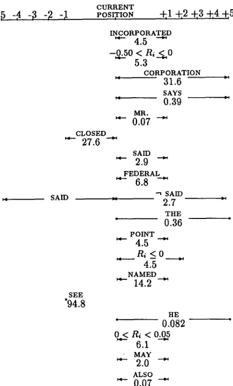
Figure 3 shows the first several features t h a t were selected by the feature induction algorithm. This shows the word or relevance score for each feature together with the value of e x for the feature after iterative scaling is complete for the final model. T h e ~-- -~ figures indicate features t h a t are active over a range of sentences. Thus, the symbol

MR. +1

I, 0.07 ,t represents the feature "Does the word MR. appear in the next sentence?" which, if true, contributes a factor of e x = 0.07 to the exponential model. Similarly, the ~ ~ figures represent features t h a t are active over a range of words. For

HE + 5

example, the figure • 0.08 • represents the question "Does the word HE appear in the next five words?" which is assigned a weight of 0.08. T h e symbol ]5 _SAID _:'.= -~ SAm +5 _{2 7} _{,I stands for a} feature which asks "Does the" word SAID appear in

the previous five sentences but

not

in the next five sentences?" and contributes a factor of 2.7 if the answer is "yes."

[image:6.612.80.306.485.617.2]

(7)

-4 -t

SAID

CURRENT

POSITION +1 + 2 +'3 +'4 +'5

INCORPORATED

~-" 4.5 -0.50 < R~..~0

5.3

CORPORATION

" 31.6 "

SAYS

" 0.39 "

MR.

~ - 0.07 "-~

CLOSED

~-" 27.6 " ~

S E E

"94.8

SAID

~ - 2.9 -'~

F E D E R A L

~-" 6.8

SAID

" 2.7

THE

• 0.36

POINT

~ - 4.5

,, , Ri _ ~ 0 ~,

4.5

NAMED

~'- 14.2 --~

HE

• 0.082

~.< Ri < 0.05 6.1

MAY

2.0 - ~

ALSO

~-- 0.07 "-~

Figure 3: First several features induced for the W S J corpus, presented in order of selection, with e x fac- tors underneath. The length of the bars indicate active range of the feature, in words or sentences, relative to the current word.

of sense. T h e first selected feature, for instance, is a strong hint t h a t an article m a y have just begun; articles in the W S J corpus often concern companies, and typically the full n a m e of the c o m p a n y (ACME

INCORPORATED, f o r instance) only appears once at the beginning of the article, and subsequently in ab- breviated f o r m (ACME). Thus the appearance of INCORPORATED is a strong indication t h a t a new article m a y have recently begun.

T h e second feature uses the relevance statistic t.

1 F o r t h e W S J e x p e r i m e n t s , we modified t h e l a n g u a g e m o d e l r e l e v a n c e s t a t i s t i c b y a d d i n g a w e i g h t t o e a c h w o r d p o s i t i o n d e p e n d i n g only o n its t r i g r a m h i s t o r y w - 2 , w - 1 . A l t h o u g h o u r r e s u l t s r e q u i r e f u r t h e r analysis, we do n o t believe t h a t t h i s m a k e s a significant difference in t h e fea-

If the trigger model performs poorly relative to the t r i g r a m model in the following sentence, this feature (roughly speaking) boosts the probability of a segment at this location by a factor of 5.3.

T h e fifth feature concerns the presence of the word MR. In hindsight, we can explain this feature by noting t h a t in W S J d a t a the style is to introduce a person in the beginning of an article by writing, for example, W I L E E . C O Y O T E , PRESIDENT OF A C M E

INCORPORATED... and then later in the article using a shortened form of the name: MR. COYOTE

CITED A LACK OF EXPLOSIVES... Thus, the presence of MR. in the following sentence discounts the probability of an article b o u n d a r y by 0.07, a factor of roughly 14.

T h e sixth feature which boosts the probability of a segment if the previous sentence contained the word CLOSED--is another artifact of the W S J domain, where articles often end with a s t a t e m e n t of a c o m p a n y ' s performance on the stock m a r k e t during the day of the story of interest. Similarly, the end of an article is often m a d e with an invitation to visit a related story; hence a sentence beginning with SEE boosts the probability of a segment b o u n d a r y by a large factor of 94.8. Since a personal pronoun typically requires an antecedent, the presence of HE a m o n g the first words is a sign t h a t the current position is not near an article boundary, and this feature therefore has a discounting factor of 0.082.

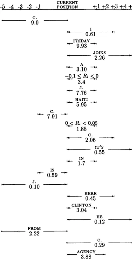
5.2 T D T f e a t u r e s

For the T D T experiments, a larger v o c a b u l a r y and roughly 800,000 candidate features were available to the induction p r o g r a m . T h o u g h the t r i g r a m prior was trained on a p p r o x i m a t e l y 150 million words, the trigger p a r a m e t e r s were trained on a 10 million word subset of the B N corpus.

Figure 4 reveals the first several features chosen by the induction algorithm. T h e letter c. a p p e a r s a m o n g several of the first features. This is because of the fact t h a t the d a t a is tokenized for speech processing (whence c. N. N. rather t h a n CNN), and the network identification information is often given at the end and beginning of news segments (c. N.

N.'S RICHARD BLYSTONE IS HERE TO TELL US...).

T h e first feature asks if the letter c. a p p e a r s in the previous five words; if so, the probability of a segment boundary is boosted by a factor of 9.0. T h e personal pronoun I appears as the second feature; if this word appears in the following three sentences then the probability of a segment b o u n d a r y is dis- counted.

T h e language model relevance statistic a p p e a r s for the first time in the sixth feature. T h e word

[image:7.612.70.299.74.453.2]

(8)

-~ -,4 -~

-7 -~t

C.

• 9 . 0

CURRENT

POSIY~ION +1 + 2 +3 +'4 +'5

I

'" 0.61 "

FRIDAY

""- 9.93 -'~

JOINS

" 2.26 " A

"-" 3.10 --0.1 < R~ < 0

3.4

J.

7.76

HAITI

~ - 5.95 " ~

C.

~-- 7.91 " ~

L< R~ < 0.0_5

1.85

C.

'~' 2.06 *'

IT ~S

J'4 Ii I

0 . 5 5 IN

~-- 1 . 7 - - ~

is ~ - 0.59 --~

Z.

0.10

FROM

2.22

HERE

'" 0.45

CLINTON

~'- 3.04 "-~

HE

" 0.12

C .

• 0.29

AGENCY

" 3.88 "'

Figure 4: First several features induced for the T D T corpus, presented in order of selection, with e ~ fac- tors underneath.

J. t h a t the seventh and fifteenth features ask a b o u t can be a t t r i b u t e d to the large n u m b e r of news stories in the d a t a having to do with the O.J. Simp- son trial. T h e nineteenth feature asks if the t e r m FROM a p p e a r s a m o n g the previous five words, and if the answer is "yes" raises the probability of a segment b o u n d a r y by more t h a n a factor of two. This feature makes sense in light of the "sign-off" conventions t h a t news reporters and anchors follow

( T H I S IS W O L F B L I T Z E R R E P O R T I N G LIVE FROM

THE WHITE

HOUSE).

Similar explanations of m a n y

of the remaining features are easy to guess f r o m a perusal of Figure 4.

6 A P r o b a b i l i s t i c E r r o r M e t r i c

Precision and recall statistics are c o m m o n l y used in natural language processing and i n f o r m a t i o n retrieval to assess the quality of algorithms. For the segmentation task they m i g h t be used to gauge how frequently boundaries actually occur when they are hypothesized and vice versa. Although they have snuck into the literature in this disguise, we believe they are unwelcome guests.

A useful error metric should somehow correlate with the utility of the i n s t r u m e n t e d procedure in a reM application. In almost any conceivable application, a segmenting tool t h a t consistently comes close--off by a sentence, s a y - - i s preferable to one t h a t places boundaries willy-nilly. Yet an a l g o r i t h m t h a t places a b o u n d a r y a sentence away f r o m the actual b o u n d a r y every t i m e actually receives w o r s e

precision and recall scores t h a n an a l g o r i t h m t h a t hypothesizes a b o u n d a r y at every position. It is natural to expect t h a t in a segmenter, close should count for something.

A useful metric should Mso be robust with respect to the scale (words, sentences, p a r a g r a p h s , for instance) at which boundaries are determined. How- ever, precision and recall are scale-dependent quan- tities. (Reynar, 1994) uses an error window t h a t redefines "correct" to m e a n hypothesized within some constant window of units away f r o m a reference boundary, b u t this approach still suffers f r o m overdiscretizing error, drawing all-or-nothing lines insensitive to gradations of correctness.

[image:8.612.76.303.76.523.2]

(9)

Our proposed metric satisfies the listed desiderata. It formalizes in a probabilistic m a n n e r the effect of d o c u m e n t co-occurrence on goodness, in which it is deemed desirable for related units of information to a p p e a r in the s a m e d o c u m e n t and unrelated units to a p p e a r in separate documents.

6.1 T h e n e w m e t r i c

Segmentation, whether at the word or sentence level, is a b o u t identifying boundaries between successive units of information in a text corpus. T w o such units are either related or unrelated by the intent of the d o c u m e n t author. A natural way to reason a b o u t developing a segmentation algorithm is therefore to optimize the likelihood t h a t two such units are correctly labeled as being related or being unrelated. Our error metric P~, is simply the probability that two sentences drawn randomly f r o m the corpus are correctly identified as belonging to the s a m e doc- u m e n t or not belonging to the s a m e document. More formally, given two segmentations r e f and hyp for a corpus n sentences long,

P , ( r e f , h y p ) = ~ D ~ ( i , j ) S r e f ( i , j ) ~ $ h y p ( i , j ) l<i<j<n

Here ~ref is an indicator function which is 1 if the two corpus indices specified by its p a r a m e t e r s belong in the s a m e document, and 0 otherwise; similarly, ~hyp is 1 if the two indices are hypothesized to belong in the same document, and 0 otherwise. T h e operator is the XNOR function ("both or neither") on its two operands. T h e function D , is a distance probability distribution over the set of possible distances between sentences chosen r a n d o m l y from the corpus, and will in general depend on certain parameters # such as the average spacing between sentences. If D~ is uniform over the length of the text, then the metric represents the probability t h a t any two sentences drawn f r o m the corpus are correctly identified as being in the s a m e document or not.

Consider the implications of this for information retrieval. Suppose there is precisely one sentence in a target corpus t h a t satisfies our information de- mands. For some applications it m a y be sufficient for the system to return only t h a t sentence, but in general we desire t h a t it return as m a n y sentences directly related to the target sentence as possible, without returning too m a n y unrelated sentences. If we assume "related" to m e a n "contained in the same d o c u m e n t " , then our error metric judges algorithms based on how often this happens.

In practice letting D~, be the uniform distribution is unreasonable, since for large corpora most r a n d o m l y drawn pairs of sentences are in different documents and are correctly identified as such by even the m o s t naive algorithms. We instead adopt

a distribution t h a t focuses on small distances. In particular, we choose D~ to be an exponential distribution with m e a n l / p , a p a r a m e t e r t h a t we fix at the a p p r o x i m a t e m e a n d o c u m e n t length for the domain:

Dt~(i, J) = 7t~ e - ~ l i - j l .

In the above, 7t, is a normalization chosen so t h a t D~, is a probability distribution over the range of distances it can accept.

There are several sanity checks t h a t validate the use of our metric. T h e measure is a probability and therefore a real n u m b e r between 0 and 1. We expect 1 to represent perfection; indeed, an algorithm scores 1 with respect to some d a t a if and only if it predicts its segmentation exactly. It captures the notion of nearness in a principled way, gently penal- izing algorithms t h a t hypothesize boundaries t h a t aren't quite right, and scaling down with the algo- r i t h m ' s degradation. Furthermore, it is not possible to "cheat" and obtain a high score with this m e t - ric: spurious behavior such as never hypothesizing boundaries and hypothesizing nothing but boundaries are penalized. We refer to Section 7 for sample results on how these trivial algorithms score.

One weakness of the metric as we have presented it here is t h a t there is no principled way of specify- ing the distance distribution Du. We plan to give a more detailed analysis of this p r o b l e m and present a m e t h o d for choosing the p a r a m e t e r s ~ in a future paper.

7 E x p e r i m e n t a l R e s u l t s

7.1 Q u a n t i t a t i v e r e s u l t s

After feature induction was carried out (as described in Section 5), a simple decision procedure was used for actually placing boundaries: a segment b o u n d a r y was placed at each position for which the model probability was above a fixed threshold or, with boundaries required to be separated by a mini- m u m n u m b e r of sentences e. T h e threshold and min- i m u m separation were determined on heldout d a t a in order to maximize the probability P~, and turned out to be a = 0.20 and e = 2 for the W S J model, and ot = 0.14 and e = 5 for the T D T models.

(10)

model

f e a t u r e i n d u c t i o n

r a n d o m

all

reference hypoth.

segments

P~

precision

757 792 83% 56%

757 757 67% 17%

757 13540 53% 5%

n o n e 757 0 52% 0%

e v e n 757 753 68% 17%

recall F.measure

54% 55

16% 17

100% 10

0%

17% 17

Table 5: Quantitative results for W S J segmentation. T h e W S J model was trained on 325K words of data, and tested on a similarly sized portion of unseen text. The top 70 features were selected. T h e mean segment length in the training and test d a t a was 1/p = 18 sentences. As a basis of comparison, the figures for several baseline models are given. T h e figures in the r a n d o m row were calculated by randomly generating a n u m b e r of segments equal to the number appearing in the test data. T h e all and n o n e rows include the figures for models which hypothesize all possible segment boundaries and no boundaries, respectively. T h e e v e n row shows the results of simply hypothesizing a segment boundary every 18 sentences.

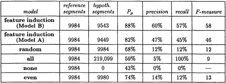
reference hypoth.

model

segments

P~

precision

f e a t u r e i n d u c t i o n

( M o d e l B) 9984 9543 88% 60% f e a t u r e i n d u c t i o n

( M o d e l A) 9984 9449 82% 47%

r a n d o m 9984 9984 68% 12%

all 9984 219,099 59% 5%

n o n e 9984 0 43% 0%

e v e n 9984 9980 74% 14%

recall F-measure

57% 58

45% 46

12% 12

100% 9

0%

12% 13

Table 6: Quantitative results for T D T segmentation. T h e T D T models were trained on 2M words and tested on 4.3M words of previously unseen T D T data. Model A was trained on 2M words of broadcast news d a t a from 1992-1993, not included in T D T corpus, and the top 100 features were selected. Model B was trained on the first 2M words of T D T corpus which is made up of a mix of CNN transcripts and Reuters newswire, and again the top 100 features were selected. The mean document length was 1 / p = 25 sentences.

assigning no boundaries, and deterministically placing a segment boundary every 1 / p sentences. It is instructive to compare the values of P , with precision and recall for these default algorithms in order to obtain some intuition for the new error metric.

Two separate models were built to segment the T D T corpus. T h e first, which we shall refer to simply as Model A, was trained using two million words from the B N corpus from the 1992-1993 time period. This d a t a contains CNN transcripts, but no Reuters newswire data. Model B was trained on the first two million words of the T D T corpus. Both models were tested on the last 4.3 million words of the T D T corpus. We expect Model A to be infe- rior to Model B for two reasons: the lack of Reuters d a t a in it's training set and the difference of between one and two years in the dates of the stories in the

training and test sets. T h e difference is quantifiied in Table 6, which shows that P~, = 0.82 for Model A while P , = 0.88 for Model B.

7.2 Q u a l i t a t i v e r e s u l t s

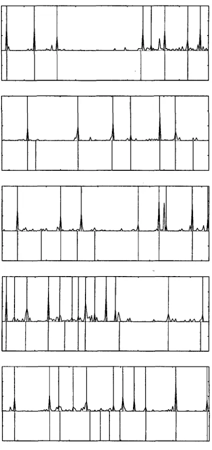
[image:10.612.106.500.70.182.2] [image:10.612.107.499.291.436.2]

(11)

h l J L ~ . - ^ . A ^ , -

I

. i

: !

!

I

. ~ . ^J

Figure 7: Typical segmentations of W S J test data. The lower verticle lines indicate reference segmentations ("truth"). The upper verticle lines are boundaries placed by the algorithm. The fluctuating curve is the probability of a segment boundary according to the exponential model after 70 features were induced.

structed using feature induction. Notice that in this domain many of the segments are quite short, adding special difficulties for the segmentation problem. Figure 8 shows the performance of the T D T segmenter (Model B) on five randomly chosen blocks of 200 sentences from the T D T test data.

We hasten to add that these results were obtained

Figure 8: Randomly chosen segmentations of T D T test data, in 200 sentence blocks, using Model B.

[image:11.612.81.291.68.513.2] [image:11.612.322.534.72.521.2]

(12)

8

_Conclusions

We have presented and evaluated a new statistical model for segmenting unpartitioned text into coherent fragments. We leverage long- and short-range language models, as well as automatic feature induction techniques, in the design of this model. In this work we rely exclusively on simple lexical features,

including a topicality measure called relevance and

a number of vocabulary features that are induced from a large space of candidate features.

We have proposed a new probabilistically motivated error metric for the assessment of segmentation algorithms. Qualitative assessment as well as the evaluation of our algorithm with this new metric demonstrates its effectiveness in two very different

domains, Wall Street Journal articles and broadcast

news transcripts.

Our immediate application of this model will be to

the video-on-demand application called Informedia

(Christel et al., 1995). We intend to mix simple audio and video features such as statistics from pauses, black frames, and color histograms with our lexical features in order to segment news broadcasts into component stories. Other applications that we have not explored in this paper include automatic infer- ence of subtopic structure for information retrieval, document summarization, and improved language modeling.

Acknowledgements

We thank Michael Witbrock and Alex Hauptmann for discussions on the segmentation problem within

the context of the Inforrnedia project. We also thank

Jalme Carbonell and Yiming Yang for their input, and for encouraging us to build segmentation models on the T D T corpus. Participants in the T D T pilot study, including James Allan, Rich Schwartz, Jon Yamron, and especially George Doddington, provided invaluable feedback on the probabilistic evaluation metric.

R e f e r e n c e s

Allan, J. To appear. Topic Detection and Tracking Corpus, Linguistic Data Consortium, University of Pennsylvania.

Beeferman, D., A. Berger, and J. Lafferty. 1997. A model of lexical attraction and repulsion. In Proceedings of the 35th Annual Meeting of the ACL, Madrid, Spain.

Berger, A., S. Della Pietra, and V. Della Pietra. 1996. A maximum entropy approach to natural

language processing. Computational Linguistics,

22(1):39-71.

Christel, M., T. Kanade, M. Mauldin, It. Iteddy, M. Sirbu, S. Stevens, and H. Wactlar. 1995. In-

formedia digital video library. Communications of

the ACM, 38(4):57-58.

Della Pietra, S., V. Della Pietra, and J. Lafferty.

1997. Inducing features of random fields. IEEE

Trans. on Pattern Analysis and Machine Intelli- gence, 19(4):380-393, April.

Hearst, M.A. 1994. Multi-paragraph segmentation of expository text. In Proceedings of the 32nd Annual Meeting of the ACL, Las Cruces, NM. Jelinek, F., B. Merialdo, S. Roukos, and M. Strauss.

1991. A dynamic language model for speech recog-

nition. In Proceedings of the DARPA Speech and

Natural Language Workshop, pp. 293-295, Febru- ary.

Katz, S. 1987. Estimation of probabilities from sparse data for the langauge model component

of a speech recognizer. IEEE Transactions on

Acoustics, Speech and Signal Processing, ASSP- 35(3):400-401, March.

Kozima, H. 1993. Text segmentation based on similarity between words, in Proceedings of the 31st Annual Meeting of the ACL, Columbus, OH, pp. 286-288.

Kozima, H. and T. Furugori. 1994. Segmenting nar-

rative text into coherent scenes. Literary and Lin-

guistic Computing, 9:13-19.

Kuhn, It. and R. de Mori. 1990. A cache-based nat-

ural language model for speech recognition. IEEE

Trans. on Pattern Analysis and Machine Intelli- gence, 12:570-583.

Lau, R., It. Rosenfeld, and S. Roukos. 1993. Adap- tive language modeling using the maximum en-

tropy principle. In Proceedings of the ARPA Hu-

man Language Technology Workshop, pages 108- 113. Morgan Kaufman Publishers.

Litman, D. J. and R. J. Passonneau. 1995. Com- bining multiple knowledge sources for discourse segmentation. In Proceedings of the 33rd Annual Meeting of the ACL, Cambridge, MA.

Neal, R. 1992. Connectionist learning of belief net-

works. Artificial Intelligence, 56:71-113.

Reynar, J. C. 1994. In Proceedings of the 32nd Annual Meeting of the ACL, student session, Las Cruces, NM.

Youmans, G. 1991. A new tool for discourse anal-

ysis: The vocabulary-management profile. Lan-