1634
Text Processing Like Humans Do:
Visually Attacking and Shielding NLP Systems
Steffen Eger†‡, Gözde Gül Şahin†‡, Andreas Rücklé†, Ji-Ung Lee†‡, Claudia Schulz†‡, Mohsen Mesgar†‡, Krishnkant Swarnkar†, Edwin Simpson†, Iryna Gurevych†‡
†Ubiquitous Knowledge Processing Lab (UKP-TUDA) ‡Research Training Group AIPHES
Department of Computer Science, Technische Universität Darmstadt
†www.ukp.tu-darmstadt.de ‡www.aiphes.tu-darmstadt.de
Abstract
Visual modifications to text are often used to obfuscate offensive comments in social media (e.g., “!d10t”) or as a writing style (“1337” in “leet speak”), among other scenar-ios. We consider this as a new type of ad-versarial attack in NLP, a setting to which hu-mans are very robust, as our experiments with both simple and more difficult visual perturba-tions demonstrate. We investigate the impact of visual adversarial attacks on current NLP systems on character-, word-, and sentence-level tasks, showing that both neural and non-neural models are, in contrast to humans, ex-tremely sensitive to such attacks, suffering per-formance decreases of up to 82%. We then explore three shielding methods—visual char-acter embeddings, adversarial training, and rule-based recovery—which substantially im-prove the robustness of the models. How-ever, the shielding methods still fall behind performances achieved in non-attack scenarios, which demonstrates the difficulty of dealing with visual attacks.
1 Introduction
For humans, visual similarity can play a decisive role for assessing the meaning of characters. Some evidence for these are: the frequent swapping of similar looking characters in Internet slang or abu-sive comments, creative trademark logos, and at-tack scenarios such as domain name spoofing (see examples in Table1).
Recently, some NLP systems have exploited vi-sual features to capture vivi-sual relationships among characters in compositional writing systems such as Chinese or Korean (Liu et al., 2017). How-ever, in more general cases, current neural NLP systems have no built-in notion of visual charac-ter similarity. Rather, they either treat characcharac-ters as discrete units forming a word or they represent characters by randomly initialized embeddings and
Internet slang writing style n00b,w!k!p3d!4, 1337 Toxic comments pi§§, ּמiggers,ḟucking Trademark logos/artwork
Domain name spoofing http://wíkipedia.org
Table 1: Examples of text in which characters have been changed to visually similar ones.
update them during training—typically in order to generate a character-based word representation that is robust to morphological variation or spelling mistakes (Ma and Hovy,2016). Intriguingly, this marked distinction between human and machine processing can be exploited as a blind spot of NLP systems. For example, spammers might send mali-cious emails or post toxic comments to online dis-cussion forums (Hosseini et al.,2017) by visually ‘perturbing’ the input text in such a way that it is
still easily recoverable by humans.
The issue of exposing and addressing the weak-nesses of deep learning models toadversarial in-puts, i.e., perturbed versions of original input sam-ples, has recently received considerable attention. For instance,Goodfellow et al.(2015) showed that small perturbations in the pixels of an image can mislead a neural classifier to predict an incorrect label for the image. In NLP,Jia and Liang(2017) inserted grammatically correct but semantically ir-relevant paragraphs to stories to fool neural read-ing comprehension models. Singh et al. (2018) showed significant drops in the performance of neural models for question answering when using simple paraphrases of the original questions.
al-legedly less damaging to human perception and un-derstanding than, e.g., syntax errors or the inser-tion of negainser-tions (Hosseini et al.,2017). 3) They do not require knowledge of the attacked model’s parameters or loss function (Ebrahimi et al.,2018).
In this work, we investigate to what extent re-cent state-of-the-art (SOTA) deep learning models are sensitive to visual attacks and explore various shielding techniques. Our contributions are:
• We introduceVIPER, a Visual Perturber that randomly replaces characters in the input with their visual nearest neighbors in a visual em-bedding space.
• We show that the performance of SOTA deep learning models substantially drops for vari-ous NLP tasks when attacked byVIPER. On individual tasks (e.g., Chunking) and attack scenarios, our observed drops are up to 82%. • We show that, in contrast to NLP systems,
hu-mans are only mildly or not at all affected by visual perturbations.
• We explore three methods to shield from visual attacks, viz., visual character embed-dings, adversarial training (Goodfellow et al.,
2015), and rule-based recovery. We quantify to which degree and in which circumstances these are helpful.
We point out that integrating visual knowledge with deep learning systems, as our visual character embeddings do, aims to make NLP models behave more like humans by taking cues directly from sen-sory information such as vision.1
2 Related Work
Our work connects to two strands of literature: ad-versarial attacks and visually informed character embeddings.
Adversarial Attacks are modifications to a clas-sifier’s input, that are designed to fool the system into making an incorrect decision, while the orig-inal meaning is still understood by a human ob-server. Different forms of attacks have been stud-ied in NLP and computer vision (CV), including at a character, syntactic, semantic and, in CV, the visual level.Ebrahimi et al.(2018) propose a char-acter flipping algorithm to generate adversarial ex-amples and use it to trick a character-level neural
1Code and data available from https://github.com/ UKPLab/naacl2019-like-humans-visual-attacks
classifier. They show that the accuracy decreases significantly after a few manipulations if certain characters are swapped. Their character flipping approach requires very strong knowledge in the form of the attacked networks’ gradients in a so-called white box attack setup. Chen et al.(2018) find that reading comprehension systems often ig-nore important question terms, thus giving incor-rect answers when these terms are replaced. Be-linkov and Bisk(2018) show that neural machine translation systems break for all kinds of noise to which humans are robust, such as reordering char-acters in words, keyboard typos and spelling mis-takes.Alzantot et al.(2018) replace words by syn-onyms to fool text classifiers. Iyyer et al. (2018) reorder sentences syntactically to generate adver-sarial examples.
In contrast to those related works which perform attacks on the character level, our attacks allow per-turbation of any character in a word while poten-tially minimizing impairment for humans. For ex-ample, the strongest attack in Belinkov and Bisk
(2018) is random shuffling of all characters, which is much more difficult to restore for humans.
To cope with adversarial attacks, adversarial training (Goodfellow et al., 2015) has been pro-posed as a standard remedy in which training data is augmented with data that is similar to the data used to attack the neural classifiers.Rodriguez and Rojas-Galeano(2018) propose simple rule-based corrections to address a limited number of attacks, including obfuscation (e.g., “idiots” to “!d10ts”) and negation (e.g., “idiots” to “NOT idiots”). Most other approaches have been explored in the context of CV, such as adding a stability objective during training (Zheng et al., 2016) and distillation ( Pa-pernot et al.,2016). However, methods to increase the robustness in CV have been shown to be less ef-fective against more sophisticated attacks (Carlini and Wagner,2017).
Visual Character Embeddings were originally proposed to address large character vocabularies in ‘compositional’ languages like Chinese and Japanese. Shimada et al.(2016) and Dai and Cai
existing work on visual character embeddings has not used visual information to attack NLP systems or to them.
3 Approach
To investigate the effects of visual attacks and pro-pose methods for shielding, we introduce 1) a vi-sual text perturber, 2) three character embedding spaces, and 3) methods for obtaining word embed-dings from character embedembed-dings, used as input representations in some of our experiments.
3.1 Text perturbations
Our visual perturberVIPERdisturbs an input text in such a way that (ideally) it is still readable by humans but causes NLP systems to fail blatantly. We parametrize VIPER by a probability p and a character embedding space, CES:2 For each char-actercin the input text a flip decision is made (i.i.d. Bernoulli distributed with probability p), and if a replacement takes place, one of up to 20 nearest neighbors in the CES is chosen.3 Thus, we denote
VIPERas taking two arguments:
VIPER=VIPER(p,CES).
Note thatVIPERis a black-box attacker as it does not require any knowledge of the attacked system. It would also be possible to design a more intel-ligent perturber that only disturbs content words (or “hot” words), similar toEbrahimi et al.(2018), but this would increase the difficulty for realizing
VIPER as a black-box attacker because different types of hot words may be relevant for different tasks.
3.2 Character Embeddings
We consider three different character embedding spaces. The first is continuous, assigning each character a dense 576 dimensional representation, which allows, e.g., for computing cosine similar-ities between any two characters as well as near-est neighbors for each input character. The other two are discrete and merely used as arguments to VIPER. Thus, they are only required to spec-ify nearest neighbors for standard input characters. For them, each charactercin a selected range (e.g., standard English alphabet a-zA-Z) is assigned a set
2CES may be any ‘embedding space’ that can be used to
identify the nearest neighbors of characters.
3The probability of choosing one of the 20 neighbors ofc
is proportional to its distance toc.
of nearest neighbors, and all nearest neighbors are equidistant toc. All three CES carry visual infor-mation, i.e., nearest neighbors are visually similar to the character in question. For practical reasons, we limit all our perturbations to the first 30k Uni-code characters throughout.
Image-based character embedding space (ICES) provides a continuous image-based char-acter embedding (ICE) for each Unicode charchar-acter. We retrieve a 24×24 image representation of the character (using Python’s PIL library), then stack the rows of this matrix (with entries between 0
and 255) to form a 24·24 = 576 dimensional embedding vector.
Description-based character embedding space (DCES) is based on the textual descriptions of Unicode characters. We first obtain descriptions of each character from the Unicode 11.0.0 final names list (e.g., latin small letter a for the character ‘a’). Then we determine a set of nearest neighbors by choosing all characters whose descriptions re-fer to the same letter in the same case, e.g., an al-ternative to latin small letter a is latin small letter a with grave as it contains the keywords small and a.
Easy character embedding space (ECES) pro-vides manually selected simple visual perturba-tions. It contains exactly one nearest neighbor for each of the 52 characters a-zA-Z, chosen as a dia-critic below or above a character, such ascˆfor the characterc.
Differences between the CESs The three em-bedding spaces play different roles in our experi-ments. We use ICES as character representations in deep learning systems. DCES and ECES are used as input toVIPER to perturb our test data.4 ECES models a ‘minimal perturbance with maxi-mal impact’ scenario: we assume that ECES per-turbations do not or only minimally affect human perception but may still have a large impact upon NLP systems. Indeed, we could have chosen an even simpler embedding space, e.g., by consider-ing visually identical characters in different alpha-bets, such as the Cyrillic ‘a’ (Unicode 1072) for a Latin ‘a’ (Unicode 97). DCES is a more difficult
4We do not attack with ICES because we also shield with
test-bed designed for evaluating our approaches un-der more realistic conditions with more varied and stronger attacks.
Table 2 exemplifies the differences between ICES, DCES, and ECES by comparing the nearest neighbors of a given character. As expected, ICES contains neighbors of characters which are merely visually similar without representing the same un-derlying character (such asΛ as a neighbor of A, orⅼas a neighbor of i). In contrast, DCES some-times has neighbors with considerable visual dis-similarity to the original character such as Cyrillic small letter i (и) which rather resembles a mirror-inverted n. The overlap between ICES and DCES is modest: out of 20 neighbors, a character has on average only four to five common neighbors in ICES and DCES.
3.3 Word Embeddings
Most neural NLP architectures encode text either on a character or word level. For the latter, word embeddings are needed. In this work, we use the ELMo architecture (Peters et al.,2018) to obtain (contextualized) word embeddings based on char-acters, i.e., there exists no fixed vocabulary and there will be no (word-level) out-of-vocabulary is-sues due to perturbation. In the following, we out-line our ELMo variant and a visual extension that includes visual signals from the input characters.
SELMo: ELMo as proposed by Peters et al.
(2018) first retrieves embeddings for every charac-ter in the input, which are learned as part of the net-work. ELMo then infers non-contextualized word embeddings by applying CNNs over all character embeddings in a word. Two layers of a deep bidi-rectional language model further process the word embeddings in their local sentential context and output contextualized word embeddings.
We slightly extend ELMo to include character embeddings for the first 30k Unicode characters (instead of the default 256). We call this variant SELMo (“Standard ELMo”). It is worth point-ing out that the learned character embeddpoint-ings of SELMo carry almost no visual information, as il-lustrated in Table 2. That is, except for a few very standard cases, nearest neighbors of charac-ters do not visually resemble the orginal characcharac-ters, even when trained on the 1 billion word benchmark (Chelba et al.,2013).5
5We believe SELMo nearest neighbors are more likely to
be Chinese/Japanese/Korean (CJK) characters because these
VELMo: To obtain a visually informed variant of ELMo, we replace learned character dings with the ICEs and keep the character embed-dings fixed during training. This means that during training, the ELMo model learns to utilize visual features of the input, thus potentially being more robust against visual attacks. We call this variant VELMo (“Visually-informed ELMo”).
To keep training times of SELMo and VELMo feasible, we use an output dimensionality of 512 instead of the original ELMo’s 1024d output. Our detailed hyperparameter setup is given in §A.1.
4 Human annotation experiment
We asked 6 human annotators, university employ-ees and students with native or near-native English language skills, to recover the original underlying English sentences given some perturbed text (data taken from the POS tagging and Chunking tasks, see Table4). We considered different conditions:
(i) clean:VIPER(0,_), i.e., no perturbation; (ii) VIPER(p,ICES)for p=0.2,0.4,0.6,0.8; (iii) VIPER(p,DCES)for p=0.2,0.4,0.6,0.8; (iv) easy:VIPER(p,ECES)for p=0.4,0.8.
For each condition, we used 60-120 sentences, where at most 20 sentences of one condition were given to an annotator. Examples of selected con-ditions are shown in Table3. Our rationale for in-cluding this recovery task is to test robustness of human perception under (our) visual perturbations. We focus on recovery instead of an extrinsic task such as POS because the latter would have required expert/trained annotators.
We evaluate by measuring the normalized edit distance between the recovered sentence and the underlying original, averaged over all sequence pairs and all human annotators. We normalize by the maximum lengths of the two sequences. In our case, this metric can be interpreted as the fraction of characters that have been, on average, wrongly recovered by human annotators. We refer to the metric as “error rate”.
Results are shown in Figure1. Ineasy, there is almost no difference between perturbation levels p=0.4and p=0.8, so we merge the two condi-tions.
Humans make copy mistakes even when the in-put is not perturbed, as evidenced by a positive
Input ICES DCES ECES SELMo e е ẹ ė ȩ є ē ę ḛ ё ë ĕ ɝ ǝ ɜ ē ě ȩ ɛ è ë ê é䟘০㣥ፔ ቼҫ↙㈘ 垀 i іⅰị ӏⅼl ļاį ḷ ĭ ѝ ȉ і ī ǐ ɪ й í ĩ î í⦙嚫 檯 爗 䈁 炾 娞 䐊 >䆳 A А Α Ạ ᾼ Ḁ Ἀ Ἁ ᾈ Λ Ʌ Ā Ӑ Ǟ А Å Ǎ Ȁ Ⱥ Á Ä Â 椖 溷 曑 呭⒏敮 瀄 ͅ唋 ⽤
Table 2: Ten nearest neighbors in our different character spaces. ‘SELMo’ refers to the nearest neighbors of the trained character embeddings in SELMo.
Condition Sentences(Perturbed / Original)
easy-0.8 Ḿř. Ĉôḟfêê iŝ â ṕřôfêŝsoř âẗ Ĉôᶅǔḿḃîâ Ĺâẘ Ŝcĥôôᶅ . Mr. Coffee is a professor at Columbia Law School .
ICES-0.6 Tṇẽ sḫսŧḋown a|fёςṱэ Э‚0ð0 wòřkếrs ḁng иllإͼũt óũṱpuէɓỳ apouț 4⁁ЗẒ0 câŗṣ : The shutdown affects 3,000 workers and will cut output by about 4,320 cars .
[image:5.595.102.494.162.262.2]DCES-0.8 Ƭʰe śƫōcƙ ɽeco⒱ɝʶȅd ṡøɯǝẅḩât ᵗö ᶂȋņìṣḣ 1 1/4 ᶪòwɇʶ áƭ 26 1/4 . The stock recovered somewhat to finish 1 1/4 lower at 26 1/4 .
Table 3: Examples of perturbed sentences and underlying originals.
easy clean .2 .4 .6 .8
Perturbation level p 0
2 4 6 8
Error rate in %
DCES ICES
Figure 1: Human annotation experiment. Error bars in-dicate std. across annotators. Foreasy, we merge the casesp=0.4/0.8.
error rate in clean. Such mistakes are typically misspellings or the wrong type of quotation marks (” vs. “). We observe a slightly higher error rate ineasythan inclean. However, on average 75% of all sentences are (exactly) correctly recovered in easywhile this number is lower (72.5%) inclean. By chance, clean contains fewer sentences with quotation marks thaneasy, for which a copy mis-take was more likely. This may explain easy’s higher error rate.
As we increase the perturbation level, the er-ror rate increases consistently for DCES/ICES. It is noteworthy that DCES perturbations are easier to parse for humans than ICES perturbations. We think this is because DCES perturbations always retain a variant of the same character, while ICES
may also disturb one character to another character (such ashtob). Another explanation is that ICES, unlike DCES and ECES, also disturbs numbers and punctuation. Numbers, especially, are more diffi-cult to recover. However, even at 80% disturbance level, humans can, on average, correctly recover at least 93% of all characters in the input text in all conditions.
In summary, humans appear very good at under-standing visual perturbations, and are almost per-fectly robust to the easy perturbations of ECES. Since adversarial attacks should have minimal im-pact on humans (Szegedy et al., 2014), the good performance of humans especially on ECES and DCES makes these two spaces ideal candidates for attacks on NLP systems.
5 Computational Experiments
We now evaluate the capabilities of SOTA neural network models to deal with visual attacks in four extrinsic evaluation tasks described in §5.1and il-lustrated in Table4. Hyperparameters of all our models are given in §A.2. We first examine the robustness of all architectures to visual perturba-tions in §5.2and then evaluate different shielding approaches in §5.3.
5.1 Tasks
[image:5.595.81.291.311.461.2]Task Task Type Input Target / Label(s) Train/Dev/Test
G2P char-lvl ẉṙḛŧϲhȩđlȳ r E < @ d 5 i 5K/1K/1K
POS word-lvl . . .exᴛêʼnᶁíng itŝ contraᶝẗ. . . . . .VBG PRP NN. . . 212K/44K/47K
Chunking word-lvl . . .exᴛêʼnᶁíng itŝ contraᶝẗ. . . . . .B-VP B-NP I-NP. . . 212K/44K/47K
[image:6.595.303.527.175.302.2]Toxic Comments sent-lvl Ḟǔĉǩ ôḟḟ , yoǔ âňtî - ŝeḿîẗîĉ ĉǔňẗ . toxic, obscene, insult 149K/10K/64K
Table 4: NLP tasks considered in this work, along with (perturbed) examples and data split statistics.
2009). We frame G2P as a sequence tagging task. To do so, we first hard-align input and output sequences using a 1-0,1-1,1-2 alignment scheme (Schnober et al.,2016) in which an input character is matched with zero, one, or two output characters. Once this preprocessing is done, input and output sequences have equal lengths and we can apply a standard BiLSTM on character-level to the aligned sequences (Reimers and Gurevych,2017).
POS & Chunking: We consider two word-level tasks. POS tagging associates each token with its corresponding word class (e.g., noun, adjec-tive, verb). Chunking groups words into syntac-tic chunks such as noun and verb phrases (NP and VP), assigning a unique tag to each word, which encodes the position and type of the syn-tactic constituent, e.g., begin-noun-phrase (B-NP). We use the training, dev and test splits provided by the CoNLL-2000 shared task (Sang and Buchholz,
2000) and use the same BiLSTM architecture as above with SELMo/VELMo embeddings.
Toxic comment (TC) classification: A very re-alistic use case for adversarial attacks is the toxic comment classification task. One could easily think of a scenario where a person with malicious intent explicitly aims to fool automated methods for detecting toxic comments or insults by obfus-cating text with non-standard characters that are still human-readable. We conduct experiments on the TC classification task provided by Kag-gle.6 It is a multi-label sentence classification task with six classes, i.e., toxic, severe toxic, ob-scene,threat,insult,identity hate. We use average SELMo/VELMo embeddings as input to an MLP.
5.2 VIPERattacks
In Figure2, we plot how various SOTA systems de-grade as we perturb the test data using DCES. We do not only include our own systems, but also ex-isting SOTA models: Marmot (Müller et al.,2013)
6
https://www.kaggle.com/c/jigsaw-toxic-comment-classification-challenge/
0 0.1 0.2 0.3 0.4 0.5 0.6 0.7 0.8 0.9 1
0 0.1 0.2 0.3 0.4 0.5 0.6 0.7 0.8 0.9
s
∗(p
)
p
POS Chunk G2P TC
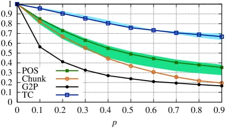
Figure 2: Degradation of SOTA systems for different perturbation levels when attacked byVIPER(p,DCES). The colored regions show how the performance of other SOTA systems relate to ours (i.e., they all suffer from similar degradation).
and Stanford POS tagger (SPT) (Manning et al.,
2014). Marmot is a feature-based POS tagger and trained on our data splits. SPT is a bi-directional dependency network tagger that mostly employs lexical features. For SPT, we used the pretrained English model provided by the toolkit. Further, we include a FastText TC classifier which has achieved SOTA performance.7 We additionally experiment with word level dependency embeddings for POS tagging and TC classification (Komninos and Man-andhar,2016).
To compare the performance of different tasks, Figure2shows scores computed by:
s∗(p) =s(p)
s(0),
where p is the perturbation level ands(p) is the score for each task at p, measured in edit distance for G2P, accuracy for POS tagging, micro-F1 for chunking, and AUCROC for TC classification. We invert the scores g of G2P by 1/g since lower scores are better for edit distance. Thus, s∗(0)is always 1 ands∗(p)is the relative performance com-pared to the clean case of no perturbations.
We see that all systems degrade considerably. For example, all three POS taggers have a perfor-mance of below 60% of the clean score when 40%
of the input characters are disturbed. Chunking de-grades even more strongly, and G2P has the highest drop: 10% perturbation level causes a 40% perfor-mance deterioration. This may be because G2P is a character-level task and the perturbation of a sin-gle character is analogous to perturbing a complete word in the word-level tasks. Finally, TC classifica-tion degrades least, i.e., only atp=0.9do we see a degradation of 30% relative to the clean score. These results appear to suggest that character-level tasks suffer the most from ourVIPERattacks and sentence-level tasks the least. However, it is worth-while pointing out that lower-bounds for individual tasks may depend on the evaluation metric (e.g., AUCROC always yields 0.5 for majority class vot-ing) as well as task-specific idiosyncrasies such as the size of the label space.
We note that the degradation curves look virtu-ally identical for both DCES or ECES perturba-tions (given in §A.3). This is in stark contrast to human performance, where ECES was much eas-ier to parse than DCES, indicating the discrepan-cies between human and machine text processing.
5.3 Shielding
We study four forms of shielding against VIPER
attacks: adversarial training (AT), visual character embeddings (CE),AT+CE, and rule-based recov-ery (RBR). ForAT, we include visually perturbed data at train time. We do not augment the training data, but replace clean examples usingVIPER in the same way as for the test data. Based on pre-liminary experiments with the G2P task, we ap-plyVIPER to the training data using ptrain=0.2. Higher levels of ptrain did not appear to improve performance. For CE, we use fixed ICEs, either fed directly into a model (G2P) or via VELMo (all other tasks). ForAT+CE, we combine adversarial training with visual embeddings. Finally, forRBR, we replace each non-standard character in the input stream with its nearest standard neighbor in ICES, where we define the standard character set as a-zA-Z plus punctuation.
Rather than absolute scores, we report differ-ences between the scores in one of the shielding treatments and original scores:
∆τ :=σ∗(p)−s∗(p), σ∗(p):=σ(p)/s(0)
whereσ(p)is the score for each task using a form of shielding. The value ∆τ denotes the improve-ment of the scores from shielding method τ over
the original scores without shielding. We normal-ize σ(p) by the score s(0) of the systems with-out shielding on clean data. We also note that our test perturbations are unseen during training for DCES; for ECES this would not make sense, be-cause each character has only one nearest neighbor. In the following, we report results mostly for DCES and show the ECES results in §A.3. We highlight marked differences between the results, however.
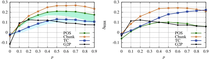
All tasks typically profit considerably fromAT
(Figure 3 left). Chunking scores improve most; e.g., atp=0.5,σ∗is 17 percent points (pp) higher than s∗. AT does not help for G2P in the DCES setting but it does help for ECES (see §A.3), where test perturbations may have been seen during train-ing. We conjecture that AT makes systems gen-erally aware that the input can be broken in some way and forces them to shield against such situa-tions, an effect similar to dropout. However, such shielding appears more difficult in character-level tasks, where a missing token is considerably more damaging than in word- or sentence-level tasks.
In Figure3(right), we observe thatCEhelps a lot for G2P, but much less particularly for POS and Chunking. We believe that for G2P, the visual char-acter embeddings restore part of the input and thus have considerable effect. It is surprising, however, that visual embeddings have no positive effect for both word-level tasks, and instead lead to small de-teriorations. A possible explanation is that, as the character embeddings are fed into the ELMo archi-tecture, their effect is dampened. Indeed, we per-formed a sanity check (see §A.5) to test how (co-sine) similar a word or sentencewis to a perturbed versionw′ ofwunder both SELMo and VELMo. We found that VELMo assigns consistently better similarities but the overall gap is small.
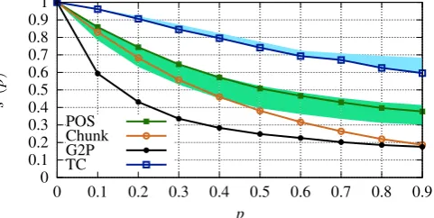
We observe that the combined effect of AT and CE (AT+CE, Figure4left) is always substantially better than either of the two alone. For instance, at p=0.5, POS improves by about 20pp, while AT alone had an effect of only 12pp and the effect of CE was even negative. Thus, it appears that AT is able to kick-start the benefits of CE, especially in the case when they alone are not effective.
RBRis excellent for ECES (see §A.3). It has a small negative effect on clean data, meaning that there is some foreign material in English texts which gets corrupted by RBR, but for any p>0
-0.1 0 0.1 0.2 0.3
0 0.1 0.2 0.3 0.4 0.5 0.6 0.7 0.8 0.9
-0.1 0 0.1 0.2 0.3
0 0.1 0.2 0.3 0.4 0.5 0.6 0.7 0.8 0.9 ∆AT
p
POS Chunk TC G2P
∆CE
p
[image:8.595.67.512.67.194.2]POS Chunk TC G2P
Figure 3: AT (with ICES replacements) and CE tested on DCES perturbed data. The colored regions show AT (with random replacements).
-0.1 0 0.1 0.2 0.3
0 0.1 0.2 0.3 0.4 0.5 0.6 0.7 0.8 0.9
-0.1 0 0.1 0.2 0.3
0 0.1 0.2 0.3 0.4 0.5 0.6 0.7 0.8 0.9 ∆AT
+
CE
p
POS Chunk TC G2P
∆RBR
p
POS Chunk TC G2P
Figure 4: AT+CE (with ICES replacements) and RBR on DCES perturbed data. The colored regions show AT (with random replacements).
than CE, even though both depend on ICES: CE in a ‘soft’ way and RBR in a ‘hard’ way. Our best explanation is that RBR is analogous to ‘machine translating’ a foreign text into English and then ap-plying a trained classifier, while CE is analogous to a direct transfer approach (McDonald et al.,2011) which trains in one domain and is then applied to another. This causes a form of domain shift to which neural nets are quite vulnerable (Ruder and Plank,2018;Eger et al.,2018a).
For DCES, RBR is outperformed by AT+CE, which better mitigates the domain shift than CE, except for TC.
We note that even with all our shielding ap-proaches, the performance of the shielded sys-tems is still considerably below the performance on clean data at some perturbation levels. E.g., at p=0.9, AT+CE shielded Chunking has a score of less than 60% of the clean performance. While it may be partially due to our character embeddings not being optimal (i.e., they assign low similarity to major and minor variants of the same letter such as ˢand s, which could be improved by size-invariant CNNs), a main reason for this could be the domain-shift induced by the perturbations, for which even
AT cannot always help when attacks are unseen during training. This is another major distinction between human and machine processing.
6 Discussion
Random AT. We discussed that the effect of AT may be similar to dropout. If so, AT with random rather than visual character replacements should be similarly effective. Indeed, the graphs in Figures3
and4show that injecting random noise generally improves the robustness, but not to the level of vi-sually informed AT (exemplarily for POS/TC).
Error analysis. We analyze the cases in which our perturbation withVIPER changes the predic-tion to a wrong class. We perform our analysis for TC as it represents a real-world attack scenario. We define the toxicity level (TL) of a commentx for a classy∈ {1, . . . ,6}and modelθ as TL(x) =
∑yθ(x,y),e.g., a commentxwhich has been clas-sified asinsult(probability 0.8) andobscene (prob-ability 0.7) gets a TL of1.5. We consider a suc-cessful attack to decrease TL after perturbation.
VIPER with DCES and p=0.1 achieves a suc-cess rate of 24.1%—i.e., roughly one fourth of the
[image:8.595.70.513.241.367.2]Perturbation (CES) Perturbed Text Toxicity Level No Shielding AT CE AT+CE RBR
clean u are a gigantic faggot 4.00 3.29 3.16 2.93 3.11 3.57
VIPER(p,ECES) u are â gigantic faggoẗ 4.00 0.11 1.05 1.37 2.05 3.57
VIPER(p,DCES) u are a ʛigantic faggoȶ 4.00 0.82 1.18 3.36 3.16 1.69
clean he is also a faggot . 4.00 3.26 3.68 2.81 2.14 3.79
VIPER(p,ECES) ĥe is also a faggot . 4.00 3.39 3.70 2.64 2.23 3.79
VIPER(p,DCES) he is alᶊo a fagᶢoƭ . 4.00 0.48 1.48 1.55 1.78 0.40
Table 5: Two examples of toxic/non-toxic comments that show the effects of the different shielding methods. We report the averaged sum over the six toxicity classes, e.g.,4.00is equal to a positive example in four classes. p=0.1.
impact on non-toxic comments is small—TL in-creased in only 3.2% of the cases.
Table 5 shows sample comments and their TL for different shielding and perturbation methods. As can be seen, perturbing specific words (hot wordsfor TC) substantially reduces the TL score of a non-shielded approach (e.g., from 3.29 to 0.11), while perturbing ‘non-hot’ words like ‘he’ has lit-tle effect. The shielding approaches help in these show-cased examples to various degrees and the shielding with AT+CE is more robust to stronger attacks (higher visual dissimilarity) than RBR.
This illustrates that a malicious attacker may aim to increase the success rate of an attack by only perturbing offensive words (in the TC task). To test whetherVIPERbenefits from perturbing such hot words, we manually compiled a list of 20 hand-selected offensive words (see §A.6) which we be-lieve are indicators of toxic comments. We then analyzed how often a perturbation of a word from this list co-occurs with a successful attack. We observe that in 55% of successful attacks, a word from our list was among the perturbed words of the comment. As our list is only a small subset of all possible offensive words, the perturbation of hot words may have an even stronger effect.
7 Conclusion
In this work, we considered visual modifications to text as a new type of adversarial attack in NLP and we showed that humans are able to reliably recover visually perturbed text. In a number of experiments on character-, word-, and sentence-level, we highlighted the fundamental differences between humans and state-of-the-art NLP systems, which sometimes blatantly fail under visual at-tack, showing that visual adversarial attacks can have maximum impact. This calls for models that have richer biases than current paradigm types do, which would allow them to bridge the gaps in infor-mation processing between humans and machines.
We have explored one such bias, visual encoding, but our results suggest that further work on such shielding is necessary in the future.
Our work is also important for system builders, such as of toxic comment detection models de-ployed by, e.g., Facebook and Twitter, who regu-larly face visual attacks, and who might face even more such attacks once visual character perturba-tions are easier to insert than via the keyboard. From the opposite viewpoint, VIPER may help users retain privacy in online engagements and when trying to avoid censorship ( Hiruncharoen-vate et al., 2015) by suggesting visually similar spellings of words.
Finally, our work shows that the ‘brittleness’ (Belinkov and Bisk,2018) of NLP extends beyond MT and beyond word reordering or replacements, a recognition that we hope inspires others to inves-tigate more ubiquitous shielding techniques.
Acknowledgments
References
Moustafa Alzantot, Yash Sharma, Ahmed Elgohary, Bo-Jhang Ho, Mani Srivastava, and Kai-Wei Chang. 2018. Generating natural language adversarial
ex-amples. In Proceedings of the 2018 Conference
on Empirical Methods in Natural Language Pro-cessing, pages 2890–2896. Association for Compu-tational Linguistics.
Yonatan Belinkov and Yonatan Bisk. 2018. Synthetic and natural noise both break neural machine transla-tion. InInternational Conference on Learning Rep-resentations.
Nicholas Carlini and David Wagner. 2017. Towards evaluating the robustness of neural networks. In
2017 IEEE Symposium on Security and Privacy, pages 39–57.
Ciprian Chelba, Tomas Mikolov, Mike Schuster, Qi Ge, Thorsten Brants, Phillipp Koehn, and Tony Robinson. 2013. One billion word benchmark for measuring
progress in statistical language modeling. Technical
report, Google.
Hongge Chen, Huan Zhang, Pin-Yu Chen, Jinfeng Yi, and Cho-Jui Hsieh. 2018. Attacking visual language grounding with adversarial examples: A case study on neural image captioning. InProceedings of the 56th Annual Meeting of the Association for Compu-tational Linguistics (Volume 1: Long Papers), vol-ume 1, pages 2587–2597.
Falcon Dai and Zheng Cai. 2017. Glyph-aware
em-bedding of chinese characters. InProceedings of
the First Workshop on Subword and Character Level Models in NLP, Copenhagen, Denmark, September 7, 2017, pages 64–69.
Timothy Dozat. 2016. Incorporating nesterov momen-tum into adam. ICLR Workshop.
Javid Ebrahimi, Anyi Rao, Daniel Lowd, and Dejing Dou. 2018.Hotflip: White-box adversarial examples
for text classification. InProceedings of the 56th
An-nual Meeting of the Association for Computational Linguistics, ACL 2018, Melbourne, Australia, July 15-20, 2018, Volume 2: Short Papers, pages 31–36.
Steffen Eger, Johannes Daxenberger, Christian Stab, and Iryna Gurevych. 2018a. Cross-lingual argumen-tation mining: Machine translation (and a bit of
pro-jection) is all you need! InProceedings of the 27th
International Conference on Computational Linguis-tics (COLING 2018).
Steffen Eger, Paul Youssef, and Iryna Gurevych. 2018b. Is it Time to Swish? Comparing Deep Learning Ac-tivation Functions Across NLP tasks. In Proceed-ings of the 2018 Conference on Empirical Methods in Natural Language Processing, pages 4415–4424. Association for Computational Linguistics.
Ian Goodfellow, Jonathon Shlens, and Christian Szegedy. 2015. Explaining and harnessing
adversar-ial examples. InInternational Conference on
Learn-ing Representations.
Chaya Hiruncharoenvate, Zhiyuan Lin, and Eric Gilbert. 2015. Algorithmically bypassing censor-ship on sina weibo with nondeterministic
homo-phone substitutions. InProceedings of the Ninth
In-ternational Conference on Web and Social Media, ICWSM 2015, University of Oxford, Oxford, UK, May 26-29, 2015, pages 150–158.
Hossein Hosseini, Sreeram Kannan, Baosen Zhang, and Radha Poovendran. 2017. Deceiving google’s perspective api built for detecting toxic comments.
arXiv preprint arXiv:1702.08138.
Mohit Iyyer, John Wieting, Kevin Gimpel, and Luke Zettlemoyer. 2018. Adversarial example generation
with syntactically controlled paraphrase networks.
InProceedings of the 2018 Conference of the North American Chapter of the Association for Computa-tional Linguistics: Human Language Technologies, Volume 1 (Long Papers), pages 1875–1885. Associ-ation for ComputAssoci-ational Linguistics.
Robin Jia and Percy Liang. 2017. Adversarial
exam-ples for evaluating reading comprehension systems.
InProceedings of the 2017 Conference on Empirical Methods in Natural Language Processing, EMNLP 2017, Copenhagen, Denmark, September 9-11, 2017, pages 2021–2031.
Alexandros Komninos and Suresh Manandhar. 2016. Dependency based embeddings for sentence classifi-cation tasks. InProceedings of the 2016 Conference of the North American Chapter of the Association for Computational Linguistics: Human Language Tech-nologies, pages 1490–1500.
Frederick Liu, Han Lu, Chieh Lo, and Graham Neu-big. 2017. Learning character-level compositionality
with visual features. InProceedings of the 55th
An-nual Meeting of the Association for Computational Linguistics, ACL 2017, Vancouver, Canada, July 30 -August 4, Volume 1: Long Papers, pages 2059–2068.
Xuezhe Ma and Eduard Hovy. 2016. End-to-end
se-quence labeling via bi-directional lstm-cnns-crf. In
Proceedings of the 54th Annual Meeting of the As-sociation for Computational Linguistics (Volume 1: Long Papers), pages 1064–1074. Association for Computational Linguistics.
Christopher D. Manning, Mihai Surdeanu, John Bauer, Jenny Finkel, Steven J. Bethard, and David Mc-Closky. 2014. The Stanford CoreNLP natural
lan-guage processing toolkit. InAssociation for
Compu-tational Linguistics (ACL) System Demonstrations, pages 55–60.
Ryan T. McDonald, Slav Petrov, and Keith B. Hall. 2011. Multi-source transfer of delexicalized
Conference on Empirical Methods in Natural Lan-guage Processing, EMNLP 2011, 27-31 July 2011, John McIntyre Conference Centre, Edinburgh, UK, A meeting of SIGDAT, a Special Interest Group of the ACL, pages 62–72.
Thomas Müller, Helmut Schmid, and Hinrich Schütze. 2013. Efficient higher-order CRFs for
morphologi-cal tagging. InProceedings of the 2013 Conference
on Empirical Methods in Natural Language Process-ing, pages 322–332, Seattle, Washington, USA. As-sociation for Computational Linguistics.
Nicolas Papernot, Patrick McDaniel, Xi Wu, Somesh Jha, and Ananthram Swami. 2016. Distillation as a defense to adversarial perturbations against deep neu-ral networks. In2016 IEEE Symposium on Security and Privacy, pages 582–597.
Matthew Peters, Mark Neumann, Mohit Iyyer, Matt Gardner, Christopher Clark, Kenton Lee, and Luke Zettlemoyer. 2018. Deep contextualized word
rep-resentations. InProceedings of the 2018 Conference
of the North American Chapter of the Association for Computational Linguistics: Human Language Tech-nologies, Volume 1 (Long Papers), pages 2227–2237. Association for Computational Linguistics.
Nils Reimers and Iryna Gurevych. 2017. Report-ing Score Distributions Makes a Difference: Perfor-mance Study of LSTM-networks for Sequence Tag-ging. In Proceedings of the 2017 Conference on Empirical Methods in Natural Language Processing (EMNLP), pages 338–348, Copenhagen, Denmark.
Korin Richmond, Robert A. J. Clark, and Susan Fitt. 2009. Robust LTS rules with the combilex speech technology lexicon. In INTERSPEECH, pages 1295–1298. ISCA.
Nestor Rodriguez and Sergio Rojas-Galeano. 2018. Shielding google’s language toxicity model against adversarial attacks. arXiv preprint arXiv:1801.01828.
Sebastian Ruder and Barbara Plank. 2018.Strong base-lines for neural semi-supervised learning under
do-main shift. InProceedings of the 56th Annual
Meet-ing of the Association for Computational LMeet-inguistics (Volume 1: Long Papers), pages 1044–1054. Associ-ation for ComputAssoci-ational Linguistics.
Erik F. Tjong Kim Sang and Sabine Buchholz. 2000.
Introduction to the conll-2000 shared task chunk-ing. InFourth Conference on Computational Natu-ral Language Learning, CoNLL 2000, and the Sec-ond Learning Language in Logic Workshop, LLL 2000, Held in cooperation with ICGI-2000, Lisbon, Portugal, September 13-14, 2000, pages 127–132.
Carsten Schnober, Steffen Eger, Erik-Lân Do Dinh, and Iryna Gurevych. 2016. Still not there? comparing traditional sequence-to-sequence models to encoder-decoder neural networks on monotone string
transla-tion tasks. InProceedings of COLING 2016, the 26th
International Conference on Computational Linguis-tics: Technical Papers, pages 1703–1714. The COL-ING 2016 Organizing Committee.
Daiki Shimada, Ryunosuke Kotani, and Hitoshi Iy-atomi. 2016. Document classification through image-based character embedding and wildcard
training. In2016 IEEE International Conference on
Big Data, BigData 2016, Washington DC, USA, De-cember 5-8, 2016, pages 3922–3927.
Sameer Singh, Carlos Guestrin, and Marco Túlio Ribeiro. 2018. Semantically equivalent adversarial
rules for debugging NLP models. InProceedings of
the 56th Annual Meeting of the Association for Com-putational Linguistics, ACL 2018, Melbourne, Aus-tralia, July 15-20, 2018, Volume 1: Long Papers, pages 856–865.
Christian Szegedy, Wojciech Zaremba, Ilya Sutskever, Joan Bruna, Dumitru Erhan, Ian Goodfellow, and Rob Fergus. 2014. Intriguing properties of neural
networks. InInternational Conference on Learning
Representations.
Stephan Zheng, Yang Song, Thomas Leung, and Ian Goodfellow. 2016. Improving the robustness of deep neural networks via stability training. In Proceed-ings of the IEEE Conference on Computer Vision and Pattern Recognition (CVPR 2016), pages 4480– 4488.
A Appendices
A.1 SELMo and VELMo Hyperparameters
Differences to the original ELMo as in (Peters et al.,2018) are:
• We exclude CNN filters of size 6 and 7. • The maximum characters per token is 20
(in-stead of 50).
• The LSTM dimensionality is 2048 (instead of 4096).
• Our projection dimensionality is 256 (instead of 512).
• We train the models for 5 epochs (instead of training it for 10 epochs).
A.2 Task Settings
randomly draw our train/dev/test splits from the whole corpus. Examples and split sizes are given in Table 4. We report edit distance between de-sired pronunciations and predicted pronunciations as metric. We report the edit distance averaged across all 1k test strings, averaged over 5 random initializations of all weight matrices.
0 0.1 0.2 0.3 0.4 0.5 0.6 0.7 0.8 0.9 1
0 0.1 0.2 0.3 0.4 0.5 0.6 0.7 0.8 0.9
s
∗(p
)
p
[image:12.595.48.289.178.299.2]POS Chunk G2P TC
Figure 5: Degradation of SOTA systems for different perturbation levels when attacked byVIPER(p,ECES). The colored regions show how the performance of other SOTA systems relate to ours.
POS & Chunking: We use the training, dev and test splits provided by the CoNLL-2000 shared task (Sang and Buchholz,2000) for both tasks. We have used a readily available LSTM-CRF sequence tagger (Reimers and Gurevych,2017) as above, but adapted for ELMo-type input embeddings, with default hyperparameter settings. We run each ex-perimental setting 10 times, and report the aver-age, measured asaccuracyfor POS andmicro-F1
for Chunking. For both tasks, we have used two stacked BiLSTM-layers with 100 recurrent units and dropout probability of0.5. Mini-batch size is chosen as 32. We used gradient clipping and early stopping to prevent overfitting. Adam is used as the optimizer.
Toxic comment classification: We use the train and test splits provided by the task organizers. For tuning our models, we split off a development set of 10k sentences from the training data. As in POS&Chunking, we train models on clean and per-turbed data using SELMo and VELMo representa-tions. We obtain the sentence representation for a single sentence by averaging ELMo word embed-dings over all tokens. We then train an MLP which we tune separately for each SELMo and VELMo embedding using random grid search with 100 dif-ferent configurations. We tune the following hy-perparameters separately for each hidden layer: the
depth of the neural network, i.e., one, two, or three hidden layers; the size of the hidden layer (128, 256, 512, or 1024); the amount of dropout after each layer (0.1 - 0.5); the activation functions for each hidden layer (tanh, sigmoid, or relu) (Eger et al., 2018b). Both models are trained for 100 epochs with an early stopping after 10 epochs with-out any substantial improvement and use Nesterov-accelerated Adaptive Moment Estimation (Dozat,
2016) for optimization. Model performance is measured as proposed by the task organizers using thearea under the receiver operating characteris-tics curve(AUCROC).
A.3 ECES Results
Figure 5 shows how the performances of various SOTA systems degrade on ECES settings. Fig-ures6and7show our shielding results on ECES perturbed data. As indicated in the main paper, RBR is able to recover ECES data almost perfectly regardless of the perturbation level. This is be-cause ECES only perturbs with a single nearest neighbor, which in addition is visually extremely similar to the underlying original, and thus, RBR can almost completely undo the perturbations.
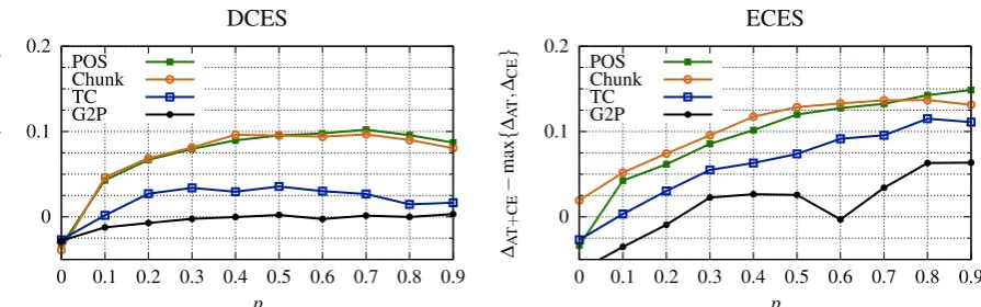
A.4 AT+CEvs.AT or CE
Figure 8 compares AT+CE against either AT or CE. For this, we compute the difference in the per-formance decrease normalized by the test perfor-mance on the clean data. As can be seen, AT+CE almost constantly outperforms either one of both, especially on word- and sentence-level tasks.
A.5 Intrinsic Evaluation
To analyze the differences between VELMo and SELMo, we investigate whether the models learn similar word embeddings for a clean sentence and its visually perturbed counterpart. We compare sentence embeddings which we obtain by averag-ing over the SELMo or VELMo word embeddaverag-ings of a sentence (clean or perturbed).
Setup Given a sentence embeddingσ of a clean sentence and an embeddingσ′ of its visually per-turbed counterpart, obtained by either averaging over VELMo (indicated by subscriptv) or SELMo (indicated by subscript s) word embeddings, we test if the condition
cos(σv,σv′)>cos(σs,σs′) (1)
-0.1 0 0.1 0.2 0.3
0 0.1 0.2 0.3 0.4 0.5 0.6 0.7 0.8 0.9
-0.1 0 0.1 0.2 0.3 0.4 0.5 0.6 0.7
0 0.1 0.2 0.3 0.4 0.5 0.6 0.7 0.8 0.9 ∆AT
p
POS Chunk TC G2P
∆CE
p
[image:13.595.72.511.105.233.2]POS Chunk TC G2P
Figure 6: AT (ICES) and CE tested on ECES perturbed data. The colored regions show AT (Random). The y axis of∆ATspans−0.15-0.3for better visualization.
-0.1 0 0.1 0.2 0.3 0.4 0.5 0.6 0.7
0 0.1 0.2 0.3 0.4 0.5 0.6 0.7 0.8 0.9
-0.1 0 0.1 0.2 0.3 0.4 0.5 0.6 0.7
0 0.1 0.2 0.3 0.4 0.5 0.6 0.7 0.8 0.9 ∆AT
+
CE
p
POS Chunk TC G2P
∆RBR
p
[image:13.595.65.510.349.472.2]POS Chunk TC
Figure 7: AT+CE (ICES) and RBR on ECES perturbed data. The colored regions show AT (Random).
0 0.1 0.2
0 0.1 0.2 0.3 0.4 0.5 0.6 0.7 0.8 0.9
0 0.1 0.2
0 0.1 0.2 0.3 0.4 0.5 0.6 0.7 0.8 0.9 ∆AT
+
CE
−
max
{
∆AT
,
∆CE
}
p
DCES
POS Chunk TC G2P
∆AT
+
CE
−
max
{
∆AT
,
∆CE
}
p
ECES
POS Chunk TC G2P
[image:13.595.63.511.564.704.2]0.6 0.7 0.8 0.9 1
0 0.2 0.4 0.6 0.8 1 -0.3 -0.2 -0.1 0 0.1 0.2 0.3 0.4 0.5 0.6
0 0.2 0.4 0.6 0.8 1 -0.3 -0.2 -0.1 0 0.1 0.2 0.3 0.4 0.5 0.6
0 0.2 0.4 0.6 0.8 1
R
p
(a)
DCES
ICES cos
(
σv
,
σ
′)v
−
cos
(
σs
,
σ
′)s
p
(b)
DCES
cos
(
σv
,
σ
′)v
−
cos
(
σs
,
σ
′)s
p
(c)
[image:14.595.68.494.52.192.2]ICES
Figure 9: Results of the intrinsic evaluation. (a) shows the ratio of cases in which the condition in Eq. (1) is met (‘R’). (b) and (c) show the average difference of the cosine similarities when sentences are perturbed with (b) DCES and (c) ICES.
For our experiments, we randomly sample 1000 sentences from the Toxic Comments dataset (see §5.1) and perturb them withVIPER(p, CES) where CES∈ {ICES, DCES}. We then count the number Nof cases in which the above condition is met with regards to the chosen CES and the value ofp, and report the ratioR=N/1000.
Results The results are given in Figure 9. In Figure 9(a) we observe that the VELMo embed-dings of a clean sentence and its perturbed coun-terpart are in many cases more similar than the ones of SELMo. For larger values of p, this ra-tio substantially increases from 70% to 95% (with ICES), which shows that VELMo is better suited to capture the similarity to the source sentence, es-pecially in cases with a strong perturbation.
In Figures 9(b) and (c) we show the (mean) difference cos(σv,σv′)−cos(σs,σs′). Here, we only observe a small positive effect in favor of VELMo, showing that the advantage of VELMo over SELMo is not substantial. We hypothesize that this is due to the contextual information which is utilized throughout the ELMo architecture, al-lowing SELMo to infer individual characters from the context of the word and the sentence. However, our results also show that the advantage of VELMo over SELMo is consistent.
Differences in similarities can also be affected by model training or the model architecture—e.g., in an extreme case a model could output the same embedding for every word/sentence. This would result in a ‘perfect’ cosine similarity, which would be advantageous in the previous experiment. Thus, we perform an additional experiment where we ex-amine if
cos(σv,σv′)>cos(σv,ρv) (2)
DCES ICES
p VELMo SELMo VELMo SELMo
0.1 0.99 0.98 1.00 0.97 0.2 0.98 0.84 0.98 0.77 0.4 0.81 0.38 0.85 0.25 0.6 0.60 0.10 0.63 0.07 0.8 0.42 0.04 0.49 0.03 1.0 0.34 0.01 0.39 0.01
Table 6: Results of the intrinsic evaluation where we compare clean sentences to their perturbed counterparts as well as randomly chosen sentences. The numbers show the ratio of cases where clean sentences are more similar to their perturbed counterparts than the ran-domly chosen sentences.
holds, where ρ is a randomly sampled sentence from the Toxic Comments dataset (with no pertur-bation). The same experiment is also performed for SELMo.
The results in Table6show that for both models with p=0.1the original sentence is in 97–100% of the cases more similar to its perturbed counter-part than the randomly chosen sentence. As the perturbation probability increases, VELMo has a clear advantage over SELMo. E.g., if we perturb all characters in a sentence (p=1.0), the SELMo embeddings of the perturbed sentence are in 1% of the cases more similar to the original sentence whereas this is the case for more than 34–39% for VELMo. Thus, VELMo embeddings better cap-ture similarity between visually similar words.
A.6 List of Hand-selected Curse Words
arrogant, ass, bastard, bitch, dick, die, fag, fat, fuck, gay, hate, idiot, jerk, kill, nigg*8, shit, stupid, suck, troll, ugly
8Due to several variations in the data, we match against
[image:14.595.325.507.255.348.2]