Hidden Variable Models for Discriminative Reranking

Hidden–Variable Models for Discriminative Reranking

Terry Koo MIT CSAIL

[email protected]

Michael Collins MIT CSAIL

[email protected]

Abstract

We describe a new method for the repre-sentation of NLP structures within rerank-ing approaches. We make use of a condi-tional log–linear model, with hidden vari-ables representing the assignment of lexi-cal items to word clusters or word senses. The model learns to automatically make these assignments based on a discrimina-tive training criterion. Training and de-coding with the model requires summing over an exponential number of hidden– variable assignments: the required sum-mations can be computed efficiently and exactly using dynamic programming. As a case study, we apply the model to parse reranking. The model gives anF– measure improvement of ≈ 1.25% be-yond the base parser, and an ≈ 0.25%

improvement beyond the Collins (2000) reranker. Although our experiments are focused on parsing, the techniques de-scribed generalize naturally to NLP struc-tures other than parse trees.

1 Introduction

A number of recent approaches in statistical NLP have focused on reranking algorithms. In rerank-ing methods, a baseline model is used to generate a set of candidate output structures for each input in training or test data. A second model, which typi-cally makes use of more complex features than the baseline model, is then used to rerank the candidates proposed by the baseline. Reranking approaches have given improvements in accuracy on a number of NLP problems including parsing (Collins, 2000; Charniak and Johnson, 2005), machine translation (Och and Ney, 2002; Shen et al., 2004), informa-tion extracinforma-tion (Collins, 2002), and natural language generation (Walker et al., 2001).

The success of reranking approaches depends critically on the choice of representation used by the

reranking model. Typically, each candidate struc-ture (e.g., each parse tree in the case of parsing) is mapped to a feature–vector representation. Previous work has generally relied on two approaches to rep-resentation: explicitly hand–crafted features (e.g., in Charniak and Johnson (2005)) or features defined through kernels (e.g., see Collins and Duffy (2002)). This paper describes a new method for the rep-resentation of NLP structures within reranking ap-proaches. We build on the intuition that lexical items in natural language often fall into word clusters (for example, president and chairman might belong to the same cluster) or fall into distinct word senses (e.g., bank might have two distinct senses). Our method involves a hidden–variable model, where the hidden variables correspond to an assignment of words to either clusters or word–senses. Lexical items are automatically assigned their hidden values using unsupervised learning within a discriminative reranking approach.

We make use of a conditional log–linear model for our task. Formally, hidden variables within the log–linear model consist of global assignments, where a global assignment entails an assignment of every word in the sentence to some hidden cluster or sense value. The number of such global assign-ments grows exponentially fast with the length of the sentence being processed. Training and decod-ing with the model requires summdecod-ing over the ex-ponential number of possible global assignments, a major technical challenge in our model. We show that the required summations can be computed ef-ficiently and exactly using dynamic–programming methods (i.e., the belief propagation algorithm for Markov random fields (Yedidia et al., 2003)) under certain restrictions on features in the model.

Previous work on reranking has made heavy use of lexical statistics, but has treated lexical items as atoms. The motivation for our method comes from the observation that statistics based on lexical items are critical, but that these statistics suffer consid-erably from problems of data sparsity and word–

sense polysemy. Our model has the ability to allevi-ate data sparsity issues by learning to assign words to word clusters, and can mitigate problems with word–sense polysemy by learning to assign lexical items to underlying word senses based upon con-textual information. A critical difference between our method and previous work on unsupervised ap-proaches to word–clustering or word–sense discov-ery is that our model is trained using a discriminative criterion, where the assignment of words to clusters or senses is driven by the reranking task in question. As a case study, in this paper we focus on syn-tactic parse reranking. We describe three model types that can be captured by our approach. The first method emulates a clustering operation, where the aim is to place similar words (e.g., president and chairman) into the same cluster. The second method emulates a refinement operation, where the aim is to recover distinct senses underlying a single word (for example, distinct senses underlying the noun bank). The third definition makes use of an existing ontol-ogy (i.e., WordNet (Miller et al., 1993)). In this case the set of possible hidden values for each word cor-responds to possible WordNet senses for the word.

In experimental results on the Penn Wall Street Journal treebank parsing domain, the hidden– variable model gives anF–measure improvement of ≈ 1.25% beyond a baseline model (the parser de-scribed in Collins (1999)), and gives an ≈ 0.25%

improvement beyond the reranking approach de-scribed in Collins (2000). Although the experiments in this paper are focused on parsing, the techniques we describe generalize naturally to other NLP struc-tures such as strings or labeled sequences. We dis-cuss this point further in Section 6.1.

2 Related Work

Various machine–learning methods have been used within reranking tasks, including conditional log– linear models (Ratnaparkhi et al., 1994; Johnson et al., 1999), boosting methods (Collins, 2000), vari-ants of the perceptron algorithm (Collins, 2002; Shen et al., 2004), and generalizations of support– vector machines (Shen and Joshi, 2003). There have been several previous approaches to parsing using log–linear models and hidden variables. Riezler et al. (2002) describe a discriminative LFG pars-ing model that is trained on standard (syntax only)

treebank annotations by treating each tree as a full LFG analysis with an observedc-structure and hid-denf-structure. Clark and Curran (2004) present an alternative CCG parsing approach that divides each CCG parse into a dependency structure (observed) and a derivation (hidden). More recently, Matsuzaki et al. (2005) introduce a probabilistic CFG aug-mented with hidden information at each nontermi-nal, which gives their model the ability to tailor it-self to the task at hand. The form of our model is closely related to that of Quattoni et al. (2005), who describe a hidden–variable model for object recog-nition in computer vision.

The approaches of Riezler et al., Clark and Cur-ran, and Matsuzaki et al. are similar to our own work in that the hidden variables are exponential in number and must be handled with dynamic– programming techniques. However, they differ from our approach in the definition of the hidden variables (the Matsuzaki et al. model is the most similar). In addition, these three approaches don’t use rerank-ing, so their features must be restricted to local scope in order to allow dynamic–programming approaches to training. Finally, these approaches use Viterbi or other approximations during decoding, something our model can avoid (see section 6.2).

In some instantiations, our model effectively clus-ters words into categories. Our approach differs from standard word clustering in that the cluster-ing criteria is directly linked to the rerankcluster-ing objec-tive, whereas previous word–clustering approaches (e.g. Brown et al. (1992) or Pereira et al. (1993)) have typically leveraged distributional similarity. In other instantiations, our model establishes word– sense distinctions. Bikel (2000) has done previous work on incorporating the WordNet hierarchy into a generative parsing model; however, this approach requires data with word–sense annotations whereas our model deals with word–sense ambiguity through unsupervised discriminative training.

3 The Hidden–Variable Model

In this section we describe a hidden–variable model based on conditional log–linear models. Each sen-tencesi for i = 1. . . n in our training data has a set ofni candidate parse treesti,1, . . . , ti,ni, which

indicating its similarity to the gold–standard parse. Without loss of generality, we define ti,1 to be the parse with the highestF–measure for sentencesi.

Given a candidate parse tree ti,j, the hidden– variable model assigns a domain of hidden val-ues to each word in the tree. For example, the hidden–value domain for the word bank could be {bank1,bank2,bank3} or {NN1,NN2,NN3}. De-tailed descriptions of the domains we used are given in Section 4.1. Formally, ifti,j spansmwords then the hidden–value domains for each word are the sets

H1(ti,j), . . . , Hm(ti,j). A global hidden–value as-signment, which attaches a hidden value to every word inti,j, is writtenh= (h1, . . . , hm)∈H(ti,j), whereH(ti,j) =H1(ti,j)×. . .×Hm(ti,j)is the set of all possible global assignments forti,j.

We define a feature–based representationΦsuch that Φ(ti,j,h) ∈ Rd is a vector of feature occur-rence counts that describes candidate parseti,j with global assignment h ∈ H(ti,j). We writeΦk for

k = 1. . . dto denote thekth _{component of the}

vec-torΦ. Each component of the feature vector is the count of some substructure within(ti,j,h). For ex-ample,Φ12andΦ101could be defined as follows:

Φ12(ti,j,h) =

Number of times the word the occurs with hidden value the3

and part of speech tagDT in (ti,j,h).

Φ101(ti,j,h) =

Number of times CEO1

ap-pears as the subject of owns2

in(ti,j,h)

(1)

We use a parameter vector Θ ∈ Rd to define a log–linear distribution over candidate trees together with global hidden–value assignments:

p(ti,j,h|si,Θ) =

eΦ(ti,j,h)·Θ

P

j0_,h0_∈H(t

i,j0)e

Φ(t_i,j0,h0_)·Θ

By marginalizing out the global assignments, we ob-tain a distribution over the candidate parses alone:

p(ti,j|si,Θ) = P

h∈H(ti,j)

p(ti,j,h|si,Θ) ₍₂₎

Later in this paper we will describe how to train the parameters of the model by minimizing the fol-lowing loss function—which is the negative log– likelihood of the training data—with respect toΘ:

L(Θ) =−P

i

logp(ti,1|si,Θ)

=−P

i

logP

h∈H(ti,1)p(ti,1,h|si,Θ)

(3)

saw with

PP(with) VP(saw)

S(saw)

a telescope NP(telescope) the boy

NP(boy) The man

NP(man)

saw

man

The the with boy

telescope

a

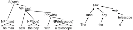
Figure 1:A sample parse tree and its dependency tree.

3.1 Local Feature Vectors

Note that the number of possible global assignments (i.e.,|H(ti,j)|) grows exponentially fast with respect to the number of words spanned byti,j. This poses a problem when training the model, or when calcu-lating the probability of a parse tree through Eq. 2. This section describes how to address this difficulty by restricting features to sufficiently local scope. In Section 3.2 we show that this restriction allows effi-cient training and decoding of the model.

The restriction to local feature–vectors makes use of the dependency structure underlying the parse treeti,j. Formally, for tree ti,j, we define the cor-responding dependency tree D(ti,j) to be a set of edges between words inti,j, where(u, v)∈D(ti,j) if and only if there is a head–modifier dependency between wordsuandv. See Figure 1 for an exam-ple dependency tree. We restrict the definition of

Φ in the following way1. If w, u and v are word indices, we introduce single–variable local feature vectorsφ(ti,j, w, hw) ∈ Rd and pairwise local fea-ture vectors φ(ti,j, u, v, hu, hv) ∈ Rd. The global feature vector Φ(ti,j,h) is then decomposed into a sum over the local feature vectors:

Φ(ti,j,h) = P 1≤w≤m

φ(ti,j, w, hw) +

P

(u,v)∈D(ti,j)

φ(ti,j, u, v, hu, hv) (4)

Notice that the second sum, over pairwise local feature vectors, respects the dependency structure D(ti,j). Section 3.2 describes how this decompo-sition ofΦleads to an efficient and exact dynamic– programming approach that, during training, allows us to calculate the gradient ∂L_∂Θ and, during testing, allows us to find the most probable candidate parse. In our implementation, each dimension of the lo-cal feature vectors is an indicator function signaling the presence of a feature, so that a sum over local feature vectors in a tree gives the occurrence count

1_{Note that the restriction on local feature vectors only}

of features in that tree. For instance, define

φ12(ti,j, w, hw) = r_h

w=the3and treeti,jassigns word

wto part–of–speechDT

z

φ101(ti,j, u, v, hu, hv) = s_(h

u, hv) = (CEO1,owns2)

and treeti,jplaces(u, v)in

a subject–verb relationship

{

where the notation JPKsignifies a0/1indicator of predicateP. When summed over the tree, these defi-nitions ofφ12andφ101yield global featuresΦ12and

Φ101as given in the previous example (see Eq. 1).

3.2 Training the Model

We now describe how the loss function in Eq. 3 can be optimized using gradient descent. The gradient of the loss function is given by:

∂L ∂Θ =−

P

i

F(ti,1,Θ) +P i,j

p(ti,j|si,Θ)F(ti,j,Θ)

whereF(ti,j,Θ) = P

h∈H(ti,j)

p(ti,j,h|si,Θ)

p(ti,j|si,Θ) Φ(ti,j,h)

is the expected value of the feature vector produced by parse treeti,j. As we remarked earlier,|H(ti,j)| is exponential in size so direct calculation of either

p(ti,j|si,Θ)orF(ti,j,Θ)is impractical. However, using the feature–vector decomposition in Eq. 4, we can rewrite the key functions ofΘas follows:

p(ti,j|si,Θ) = PZi,j

j0Zi,j0

F(ti,j,Θ) =

P

1≤w≤m hw∈Hw(ti,j)

p(ti,j, w, hw)φ(ti,j, w, hw) +

P

(u, v)∈D(ti,j)

hu∈Hu(ti,j)

hv∈Hv(ti,j)

p(ti,j, u, v, hu, hv)φ(ti,j, u, v, hu, hv)

where p(ti,j, w, hw) and p(ti,j, u, v, hu, hv) are marginalized probabilities andZi,jis the associated normalization constant:

Zi,j = P

h∈H(ti,j)

eΦ(ti,j,h)·Θ

p(ti,j, w, x) = P

h|hw=x

p(ti,j,h|si,Θ)

p(ti,j, u, v, x, y) = P

h|hu=x,hv=y

p(ti,j,h|si,Θ)

The three quantities above can be computed with be-lief propagation (Yedidia et al., 2003), a dynamic– programming technique that is efficient2 and exact

2_{The running time of belief propagation varies linearly with}

the number of nodes inD(ti,j)and quadratically with the

car-dinality of the largest hidden–value domain.

when the graph D(ti,j) is a tree, which is the case in our parse reranking model. Having calculated the gradient in this way, we minimize the loss using stochastic gradient descent3(LeCun et al., 1998).

4 Features for Parse Reranking

The previous section described hidden–variable models for discriminative reranking. We now de-scribe features for the parse reranking problem. We focus on the definition of hidden–value domains and local feature vectors in the reranking model.

4.1 Hidden–Value Domains and Local Features

Each word in a parse tree is given a domain of pos-sible hidden values by the hidden–variable model. Models with widely varying behavior can be created by changing the way these domains are defined. In particular, in this section we will see how different definitions of the domains give rise to the three main model types: clustering, refinement, and mapping into a pre–built ontology such as WordNet.

As illustration, consider a simple approach that splits each word into a domain of three word–sense hidden values (e.g., the word bank would yield the domain {bank1,bank2,bank3}). In this approach, each word receives a domain of hidden values that is not shared with any other word. The model is then able to distinguish several different usages for each word, emulating a refinement operation. An alternative approach is to split each word’s part–of– speech tag into several sub–tags (e.g., bank would yield{NN₁,NN₂,NN₃}). This approach assigns the same domain to many words; for instance, singular nouns such as bond, market, and bank all receive the same domain. The behavior of the model then emu-lates a clustering operation.

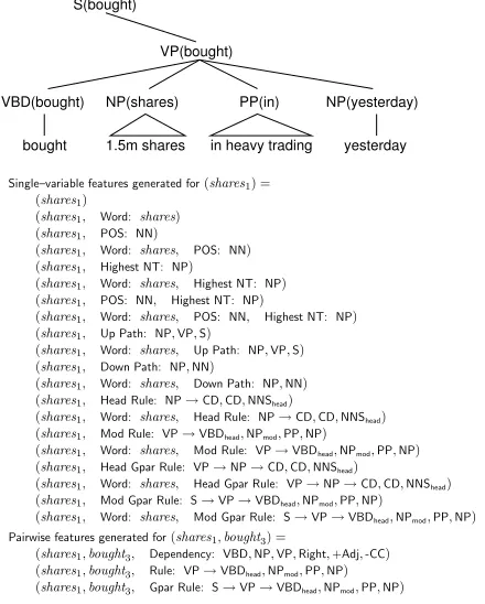
Figure 2 shows the single–variable and pairwise features used in our experiments. The features are shown with hidden variables corresponding to word–specific hidden values, such as shares1 or bought₃. In our experiments, we made use of fea-tures such as those in Figure 2 in combination with the following four definitions of the hidden–value

3

bought 1.5m shares in heavy trading yesterday VBD(bought) NP(shares) PP(in) NP(yesterday)

S(bought)

VP(bought) PSfrag replacements

Pairwise features generated for(shares1,bought3) =

(shares1,bought3, Dependency: VBD,NP,VP,Right,+Adj,-CC) (shares1,bought3, Rule: VP→VBDhead,NPmod,PP,NP) (shares1,bought3, Gpar Rule: S→VP→VBDhead,NPmod,PP,NP) Single–variable features generated for(shares1) =

(shares1)

(shares1, Word: shares) (shares1, POS: NN)

(shares1, Word: shares, POS: NN) (shares1, Highest NT: NP)

(shares1, Word: shares, Highest NT: NP) (shares1, POS: NN, Highest NT: NP)

(shares1, Word: shares, POS: NN, Highest NT: NP) (shares1, Up Path: NP,VP,S)

(shares1, Word: shares, Up Path: NP,VP,S) (shares1, Down Path: NP,NN)

(shares1, Word: shares, Down Path: NP,NN) (shares1, Head Rule: NP→CD,CD,NNShead)

(shares1, Word: shares, Head Rule: NP→CD,CD,NNShead) (shares1, Mod Rule: VP→VBDhead,NPmod,PP,NP)

(shares1, Word: shares, Mod Rule: VP→VBDhead,NPmod,PP,NP) (shares1, Head Gpar Rule: VP→NP→CD,CD,NNShead)

(shares1, Word: shares, Head Gpar Rule: VP→NP→CD,CD,NNShead) (shares1, Mod Gpar Rule: S→VP→VBDhead,NPmod,PP,NP)

(shares1, Word: shares, Mod Gpar Rule: S→VP→VBDhead,NPmod,PP,NP)

Figure 2: The features used in our model. We

show the single–variable features produced for hidden value

shares1 and the pairwise features produced for hidden values

(shares1,bought3), in the context of the given parse fragment.

Highest NT= highest nonterminal,Up Path= sequence of

ances-tor nonterminals,Down Path= sequence of headed nonterminals,

Head Rule= rules headed by the word,Mod Rule= rule in which

word acts as modifier,Head/Mod Gpar Rule=Head/Mod Ruleplus grandparent nonterminal.

domains (in each case we give the model type that results from the definition—clustering, refinement, or pre–built ontology—in parentheses):

Lexical (Refinement) Each word is split into three sub–values. See Figure 2 for an example of features generated for this choice of domain.

Part–of–Speech (Clustering) The part–of– speech tag of each word is split into five sub–values. In Figure 2, the word shares would be assigned the domain{NNS1, . . . ,NNS5}, and the word bought would have the domain{VBD1, . . . ,VBD5}.

Highest Nonterminal (Clustering) The high-est nonterminal to which each word propagates as a headword is split into five sub–values. In Figure 2 the word bought yields domain{S₁, . . . ,S₅}, while in yields{PP1, . . . ,PP5}.

Supersense (Pre–Built Ontology) We borrow the idea of using WordNet lexicographer filenames as broad “supersenses” from Ciaramita and John-son (2003). For each word, we split each of its

supersenses into three sub–supersenses. If no su-persenses are available, we fall back to splitting the part–of–speech into five sub–values. For ex-ample, shares has the supersenses noun.possession, noun.act and noun.artifact, which yield the do-main{noun.possession₁,noun.act₁,noun.artifact₁, . . .

noun.possession₃,noun.act₃,noun.artifact₃}. On the other hand, in does not have any WordNet super-senses, so it is assigned the domain{IN₁, . . . ,IN₅}. 4.2 The Final Feature Sets

We created eight feature sets by combining the four hidden–value domains above with two alterna-tive definitions of dependency structures: standard head–modifier dependencies and “sibling dependen-cies.” When using sibling dependencies, connec-tions are established between the headwords of ad-jacent siblings. For instance, the head–modifier dependencies produced by the tree fragment in Figure 2 are (bought,shares), (bought,in), and

(bought,yesterday), while the corresponding sibling dependencies are(bought,shares),(shares,in), and

(in,yesterday). 4.3 Mixed Models

The different hidden–variable models display vary-ing strengths and weaknesses. We created mixtures of different models using a weighted average:

logp(ti,j|si) = M

X

m=1

λmlogpm(ti,j|si,Θm)−Z(si)

whereZ(si)is a normalization constant that can be ignored, as it does not affect the ranking of parses. The λm weights are determined through optimiza-tion of parsing scores on a development set.

5 Experimental Results

We trained and tested the model on data from the Penn Treebank (Marcus et al., 1994). Candidate parses were produced by an N–best version of the Collins (1999) parser. Our training data consists of Treebank Sections 2–21, divided into a training cor-pus of 35,540 sentences and a development corcor-pus of 3,676 sentences. In later experiments, we made use of a secondary development corpus of 1,914 sen-tences from Section 0. Sections 22–24, containing 5,455 sentences, were held out as the test set.

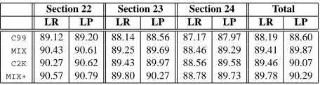
Section 22 Section 23 Section 24 Total LR LP LR LP LR LP LR LP

C99 89.12 89.20 88.14 88.56 87.17 87.97 88.19 88.60

MIX 90.43 90.61 89.25 89.69 88.46 89.29 89.41 89.87

C2K 90.27 90.62 89.43 89.97 88.56 89.58 89.46 90.07

MIX+ 90.57 90.79 89.80 90.27 88.78 89.73 89.78 90.29

Table 1:The results on Sections 22–24. LR = Labeled Recall,

LP = Labeled Precision.

method to optimize the parameters of the model. We created various mixtures of the eight models using the weighted–average technique described in Sec-tion 4.3, testing the accuracy of each mixture on the secondary development set. Our final model was a mixture of three of the eight possible models: super-sense hidden values with sibling trees, lexical hid-den values with sibling trees, and highest nontermi-nal hidden values with normal head–modifier trees.

Our final tests evaluated four models. The two baseline models are the Collins (1999) base parser, C99, and the Collins (2000) reranker,C2K. The first new model is the MIX model, which is a combina-tion of the C99 base model with the three models described above. The second new model, MIX+, is created by augmenting MIX with features from the method in C2K. Table 1 shows the results. The MIX model obtains an F–measure improvement of ≈1.25%over theC99baseline, an improvement that is comparable to theC2Kreranker. TheMIX+model yields an improvement of≈0.25%beyondC2K.

We tested the significance of 8 comparisons cor-responding to the results in Table 1 using the sign test4: we testedMIXvs.C99on Sections 22, 23, and 24 individually, as well as on Sections 22–24 taken as a whole; we also testedMIX+vs.C2K on these 4 test sets. Of the 8 comparisons, all showed signif-icant improvements at the level p ≤ 0.01 with the exception of one test,MIX+vs.C2Kon Section 24.

6 Discussion

6.1 Applying the Model to Other NLP Tasks

In this section, we discuss how hidden–variable models might be applied to other NLP problems, and in particular to structures other than parse trees. To

4

The input to the sign test is a set of sentences with judge-ments for each sentence indicating whether model 1 gives a better parse than model 2, model 2 gives a better parse than model 1, or models 1 and 2 give equal quality parses. When using the sign test, for each sentence in question we calculate theF–measure at the sentence level for the two models being compared, deriving the required judgement from these scores.

summarize the model, the major components of the approach are as follows:

•We assume some set of candidate structuresti,j, which are to be reranked by the model. Each struc-tureti,jhasni,jwordsw1, . . . , wni,j, and each word

wkhas a setHk(ti,j)of possible hidden values.

•We assume a graphD(ti,j)for eachti,j that de-fines possible interactions between hidden variables in the model. We assume some definition of local feature vectors, which consider either single hidden variables, or pairs of hidden variables that are con-nected by an edge inD(ti,j).

The approach can be instantiated in several ways when applying the model to other NLP tasks. We have already seen that by changing the definition of the hidden–value domains Hk(ti,j), we can de-rive models with widely varying behavior. In ad-dition, there is no requirement that the hidden vari-ables only be associated with words in the structure; the hidden variables could be associated with other units. For example, in speech recognition hidden variables could be associated with phonemes rather than words, and in Chinese word segmentation, hid-den variables could be associated with individual characters rather than words.

NLP tasks other than parsing involve structures

ti,jthat are not necessarily parse trees. For example, in speech recognition candidates are simply strings (utterances); in tagging tasks candidates are labeled sequences (e.g., sentences labeled with part–of– speech tag sequences); in machine translation can-didate structures may be source–language/target– language pairs, along with alignment structures specifying the correspondence between words in the two languages. Sentences and labeled sequences are in a sense simplifications of the parsing case, where a natural choice for the underlying graph D(ti,j) would be anNth_{order Markov structure, where each}

6.2 Packed Representations and Locality

One natural extension of our reranker is to adapt it to candidate parses represented as a packed parse for-est, so that it can operate on the base parser’s full output instead of a limited N-best list. However, as we described in Section 3.1, our features are lo-cally scoped with respect to hidden–variable interac-tions but unrestricted regarding information derived from the underlying candidate parses, which poses a problem for the use of packed representations. For instance, the Up/Down Pathfeatures (see Figure 2) enumerate the vertical sequences of nontermi-nals that extend above and below a given headword. We could restrict the features to local scope on the candidate parses, allowing dynamic–programming to be used to train the model with a packed rep-resentation. However, even with these restrictions, finding arg maxtPhp(t,h|s,Θ) is NP–hard, and

the Viterbi approximation arg maxt,hp(t,h|s,Θ)

— or other approximations — would have to be used (see Matsuzaki et al. (2005)).

6.3 Empirical Analysis of the Hidden Values

Our model makes no assumptions about the interpre-tation of the hidden values assigned to words: dur-ing traindur-ing, the model simply learns a distribution over global hidden–value assignments that is useful in improving the log–likelihood of the training data. Intuitively, however, we expect that the model will learn to make hidden–value assignments that are rea-sonable from a linguistic standpoint. In this section we describe some empirical observations concern-ing hidden values assigned by the model.

We established a corpus of parse trees with hidden–value annotations, as follows. First, we find the optimal parametersΘ∗ on the training set. For every sentence si in the training set, we then use

Θ∗to findt∗_i, the most probable candidate parse un-der the model. Finally, we use Θ∗ to decode h∗_i, the most probable global assignment of hidden val-ues, for each parse treet∗_i. We created a corpus of

(t∗_i,h∗_i)pairs for the feature set defined by part–of– speech hidden–value domains and standard depen-dency structures. The remainder of this section de-scribes trends for several of the most common part– of–speech categories in the corpus.

As a first example, consider the hidden values for the part–of–speech VB(infinitival verb). In the

majority of cases, words taggedVBeither modify a modal verb taggedMD(e.g., in the new rate will/MD

be/VBpayable) or the infinitival marker to (e.g., in in an effort to streamline/VBbureaucracy). The statis-tics of our corpus reflect this distinction. In 11,546 cases of the VB₁ hidden value, 10,652 cases mod-ified to, and 81 cases modmod-ified modals taggedMD. In contrast, in 11,042 cases of the VB2 value, the numbers were 8,354 and 599 for modification of modals and to respectively, showing the opposite preference. This polarization of hidden values al-lows modifiers to theVB (e.g., payable in the new rate will be payable) to be sensitive to whether the verb is modifying a modal or to.

In a related case, the hidden values for the part– of–speech TO (corresponding to the word to) also show that the model is learning useful structure. Consider cases where to heads a clause which may or may not have a subject (e.g., in it expectshits sales to remain steadyivs. a proposalhto ease reporting requirementsi). We find that for hidden values TO₁ andTO₅ together, 946 out of 976 cases have a sub-ject. In contrast, for the hidden valueTO₄, only 29 out of 10,148 cases have a subject. This splitting of theTOpart–of–speech allows modifiers to to, or words modified by to, to be sensitive to the presence or absence of a subject in the clause headed by to.

Finally, consider the hidden values for the part– of–speechNNS(plural noun). In this case, the model distinguishes contexts where a plural noun acting as the head of a noun–phrase is or isn’t modified by a post–modifier (such as a prepositional phrase or rel-ative clause). For hidden value NNS3, 12,003 out of the 12,664 instances in our corpus have a post– modifier, but for hidden valueNNS₅, only 4,099 of the 39,763 occurrences have a post–modifier. Sim-ilar contextual effects were observed for other noun categories such as singular or proper nouns.

7 Conclusions and Future Research

the hidden–variable model achieves reranking per-formance comparable to the reranking approach de-scribed by Collins (2000), and the two rerankers can be combined to yield an additive improvement.

Future work may consider the use of hidden– value domains with mixed contents, such as a do-main that contains 3 refinement–oriented lexical ues and 3 clustering–oriented part–of–speech val-ues. These mixed values would allow the hidden– variable model to exploit interactions between clus-tering and refinement at the level of words and de-pendencies. Another area for future research is to investigate the use of unlabeled data within the ap-proach, for example by making use of clusters de-rived from large amounts of unlabeled data (e.g., see Miller et al. (2004)). Finally, future work may apply the models to NLP tasks other than parsing.

Acknowledgements

We would like to thank Regina Barzilay, Igor Malioutov, and Luke Zettlemoyer for their many comments on the paper. We gratefully acknowl-edge the support of the National Science Founda-tion (under grants 0347631 and 0434222) and the DARPA/SRI CALO project (through subcontract No. 03-000215).

References

Daniel Bikel. 2000. A statistical model for parsing and word– sense disambiguation. In Proceedings of EMNLP.

Peter F. Brown, Vincent J. Della Pietra, Peter V. deSouza, Jen-nifer C. Lai, and Robert L. Mercer. 1992. Class–basedn– gram models of natural language. Computational Linguis-tics, 18(4):467–479.

Eugene Charniak and Mark Johnson. 2005. Coarse–to–finen– best parsing and maxent discriminative reranking. In

Pro-ceedings of the 43rdACL.

Massimiliano Ciaramita and Mark Johnson. 2003. Supersense tagging of unknown nouns in wordnet. In EMNLP 2003.

Stephen Clark and James R. Curran. 2004. Parsing the wsj using ccg and log–linear models. In ACL, pages 103–110.

Michael Collins and Nigel Duffy. 2002. New ranking algo-rithms for parsing and tagging: Kernels over discrete struc-tures, and the voted perceptron. In ACL 2002.

Michael Collins. 1999. Head–Driven Statistical Models for

Natural Language Parsing. Ph.D. thesis, University of

Pennsylvania, Philadelphia, PA.

Michael Collins. 2000. Discriminative reranking for natural language parsing. In Proceedings of the 17th_ICML.

Michael Collins. 2002. Ranking algorithms for named entity extraction: Boosting and the voted perceptron. In ACL 2002.

Robert G. Cowell, A. Philip Dawid, Steffen L. Lauritzen, and David J. Spiegelhalter. 1999. Probabilistic Networks and Expert Systems. Springer.

Mark Johnson, Stuart Geman, Stephen Canon, Zhiyi Chi, and Stefan Riezler. 1999. Estimators for stochastic “unification– based” grammars. In Proceedings of the 37th_ACL.

Y. LeCun, L. Bottou, Y. Bengio, and P. Haffner. 1998. Gradient–based learning applied to document recognition. Proceedings of the IEEE, 86(11):2278–2324, November.

Mitchell P. Marcus, Beatrice Santorini, and Mary Ann Marcinkiewicz. 1994. Building a large annotated corpus of english: The penn treebank. Computational Linguistics, 19(2):313–330.

Takuya Matsuzaki, Yusuke Miyao, and Jun’ichi Tsujii. 2005. Probabilistic cfg with latent annotations. In ACL.

George A. Miller, Richard Beckwith, Christiane Fellbaum, Derek Gross, and Katherine Miller. 1993. Five papers on wordnet. Technical report, Stanford University.

Scott Miller, Jethran Guinness, and Alex Zamanian. 2004. Name tagging with word clusters and discriminative train-ing. In HLT–NAACL, pages 337–342.

Franz Josef Och and Hermann Ney. 2002. Discriminative train-ing and maximum entropy models for statistical machine translation. In Proceedings of the 40thACL, pages 295–302.

Fernando C. N. Pereira, Naftali Tishby, and Lillian Lee. 1993. Distributional clustering of english words. In Proceedings

of the 31stACL, pages 183–190.

Ariadna Quattoni, Michael Collins, and Trevor Darrell. 2005. Conditional random fields for object recognition. In NIPS 17. MIT Press.

Adwait Ratnaparkhi, Salim Roukos, and R. Todd Ward. 1994. A maximum entropy model for parsing. In ICSLP 1994.

Stefan Riezler, Tracy H. King, Ronald M. Kaplan, Richard S. Crouch, John T. Maxwell III, and Mark Johnson. 2002. Parsing the wall street journal using a lexical–functional grammar and discriminative estimation techniques. In ACL.

Libin Shen and Aravind K. Joshi. 2003. An svm–based vot-ing algorithm with application to parse rerankvot-ing. In Walter Daelemans and Miles Osborne, editors, Proceedings of the

7thCoNLL, pages 9–16. Edmonton, Canada.

Libin Shen, Anoop Sarkar, and Franz Josef Och. 2004. Dis-criminative reranking for machine translation. In HLT– NAACL, pages 177–184.

Marilyn A. Walker, Owen Rambow, and Monica Rogati. 2001. Spot: A trainable sentence planner. In NAACL.