A Plethora of Methods for Learning English Countability
Timothy Baldwin CSLI Stanford University Stanford, CA 94305 USA
Francis Bond
NTT Communication Science Laboratories Nippon Telegraph and Telephone Corporation
Kyoto, Japan
Abstract
This paper compares a range of methods for classifying words based on linguis-tic diagnoslinguis-tics, focusing on the task of learning countabilities for English nouns. We propose two basic approaches to feature representation: distribution-based representation, which simply looks at the distribution of features in the cor-pus data, and agreement-based represen-tation which analyses the level of token-wise agreement between multiple pre-processor systems. We additionally com-pare a single multiclass classifier archi-tecture with a suite of binary classifiers, and combine analyses from multiple pre-processors. Finally, we present and evalu-ate a feature selection method.
1 Introduction
Lexical acquisition can be described as the process of populating a grammar skeleton with lexical items, through a process of mapping word lemmata onto lexical types described in the grammar. Depending on the linguistic precision of the base grammar, lex-ical acquisition can range in complexity from sim-ple part-of-speech tagging (shallow lexical
acquisi-tion) to the acquisition of selectionally-constrained
subcategorisation frame clusters or constructional compatibilities (deep lexical acquisition). Our par-ticular interest is in the latter task of deep lexical acquisition with respect to English nouns.
We are interested in developing learning tech-niques for deep lexical acquisition which take a fixed set of linguistic diagnostics, and classify words ac-cording to corpus data. We propose a range of gen-eral techniques for this task, as exemplified over the task of English countability acquisition. Countabil-ity is the syntactic property that determines whether a noun can take singular and plural forms, and af-fects the range of permissible modifiers. Many nouns have both countable and uncountable lemmas,
with differences in meaning: I submitted two papers “documents” (countable) vs. Please use white paper “substance to be written on” (uncountable).
This research complements that described in Baldwin and Bond (2003), where we present the lin-guistic foundations and features drawn upon in the countability classification task, and motivate the claim that countability preferences can be learned from corpus evidence. In this paper, we focus on the methods used to tackle the task of countability classification based on this fixed feature set.
The remainder of this paper is structured as fol-lows. Section 2 outlines the countability classes, resources and pre-processors. Section 3 presents two methods of representing the feature space. Sec-tion 4 details the different classifier designs and the dataset, which are then evaluated in Section 5. Fi-nally, we conclude the paper with a discussion in Section 6.
2 Preliminaries
In this section, we describe the countability classes, the resources used in this research, and the feature extraction method. These are described in greater detail in Baldwin and Bond (2003).
2.1 Countability classes
Nouns are classified as belonging to one or more of four possible classes: countable, uncountable, plural only and bipartite. Countable nouns can be modi-fied by denumerators, prototypically numbers, and have a morphologically marked plural form: one
dog, two dogs. Uncountable nouns cannot be
mod-ified by denumerators, but can be modmod-ified by un-specific quantifiers such as much; they do not show any number distinction (prototypically being singu-lar): *one equipment, some equipment, *two
equip-ments. Plural only nouns only have a plural form,
such as goods, and cannot be either denumerated or modified by much; many plural only nouns, such as clothes, use the plural form even as modifiers: a
clothes horse. Bipartite nouns are plural when they
be denumerated with the classifier pair: a pair of
scissors.
2.2 Gold standard data
Information about noun countability was obtained from two sources: COMLEX 3.0 (Grishman et al., 1998) and the common noun part of ALT-J/E’s Japanese-to-English semantic transfer dictio-nary (Ikehara et al., 1991). Of the approximately 22,000 noun entries inCOMLEX, 13,622 are marked as countable, 710 as uncountable and the remainder are unmarked for countability. ALT-J/E has 56,245 English noun types with distinct countability.
2.3 Feature space
Features used in this research are divided up into
feature clusters, each of which is conditioned on
the occurrence of a target noun in a given construc-tion. Feature clusters are either one-dimensional (describing a single multivariate feature) or two-dimensional (describing the interaction between two multivariate features), with each dimension describ-ing a lexical or syntactic property of the construc-tion in quesconstruc-tion. An example of a one-dimensional feature cluster is head noun number, i.e. the num-ber (singularorplural) of the target noun when it oc-curs as the head of an NP; an example of a two-dimensional feature cluster in subject–verb agree-ment, i.e. the number (singular orplural) of the tar-get noun when it occurs as head of a subject NP vs. number agreement on the verb (singular or plu-ral). Below, we provide a basic description of the 10 feature clusters used in this research and their di-mensionality ([x]=1-dimensional feature cluster with x unit features,[x×y]=2-dimensional feature cluster withx×yunit features). These represent a total of 206 unit features.
Head noun number:[] the number of the target noun when it heads an NP
Modifier noun number:[] the number of the target noun when a modifier in an NP
Subject–verb agreement:[×] the number of the target noun in a subject position vs. number agreement on the governing verb
Coordinate noun number:[×] the number of the target noun vs. the number of the head nouns of conjuncts
N of N constructions:[×] the type of the N(e.g.
COLLECTIVE, TEMPORAL) vs. the number of the
target noun (N) in an Nof Nconstruction
Occurrence in PPs:[×] the preposition type vs.
the presence or absence of a determiner when the target noun occurs in singular form in a PP
Pronoun co-occurrence:[×] what personal, pos-sessive and reflexive pronouns (e.g. he, their,
itself ) occur in the same sentence as singular
and plural instances of the target noun
Singular determiners:[] what singular-selecting determiners (e.g. a, much) occur in NPs headed by the target noun in singular form
Plural determiners:[] what plural-selecting de-terminers (e.g. many, various) occur in NPs headed by the target noun in plural form
Non-bounded determiners:[×] what non-bounded determiners (e.g. more, sufficient) occur in NPs headed by the target noun, and what is the number of the target noun for each
2.4 Feature extraction
The values for the features described above were ex-tracted from the written component of the British National Corpus (BNC, Burnard (2000)) using three different pre-processors: (a) a POS tagger, (b) a full-text chunker and (c) a dependency parser. These are used independently to test the efficacy of the differ-ent systems at capturing features used in the clas-sification process, and in tandem to consolidate the strengths of the individual methods.
With the POS extraction method, we first tagged the BNC using an fnTBL-based tagger (Ngai and Florian, 2001) trained over the Brown and WSJ cor-pora and based on the Penn POS tagset. We then lemmatised this data using a Penn tagset-customised version of morph (Minnen et al., 2001). Finally, we implemented a range of high-precision, low-recall POS-based templates to extract out the features from the processed data.
For the chunker, we ran fnTBL over the lem-matised tagged data, training over CoNLL 2000-style (Tjong Kim Sang and Buchholz, 2000) chunk-converted versions of the full Brown and WSJ cor-pora. For the NP-internal features (e.g. determin-ers, head number), we used the noun chunks directly, or applied POS-based templates locally within noun chunks. For inter-chunk features (e.g. subject–verb agreement), we looked at only adjacent chunk pairs so as to maintain a high level of precision.
We read dependency tuples directly off the output of RASP (Briscoe and Carroll, 2002b) in grammati-cal relation mode.1 RASP has the advantage that re-call is high, although precision is potentially lower
1
than chunking or tagging as the parser is forced into resolving phrase attachment ambiguities and com-mitting to a single phrase structure analysis.
After generating the different feature vectors for each noun based on the above configurations, we fil-tered out all nouns which did not occur at least 10 times in NP head position in the output of all three systems. This resulted in a total of 20,530 nouns, of which 9,031 are contained in the combined COM-LEXandALT-J/Elexicons. The evaluation is based on these 9,031 nouns.
3 Feature representation
We test two basic feature representations in this re-search: distribution-based, which simply looks at the relative occurrence of different features in the corpus data, and agreement-based, which analyses the level of token-wise agreement between multiple systems.
3.1 Distribution-based feature representation
In the distribution-based feature representation, we take each target noun in turn and compare its amal-gamated value for each unit feature with (a) the val-ues for other target nouns, and (b) the value of other unit features within that same feature cluster. That is, we focus on the relative prominence of features globally within the corpus and locally within each feature cluster.
In the case of a one-dimensional feature cluster (e.g. singular determiners), each unit featurefs for target noun w is translated into 3 separate feature values:
corpfreq(fs,w) =
freq(fs|w)
freq(∗) (1)
wordfreq(fs,w) =
freq(fs|w)
freq(w) (2)
featfreq(fs,w) =
freq(fs|w) P
ifreq(fi|w)
i (3)
wherefreq(∗)is the frequency of all words in the cor-pus. That is, for each unit feature we capture the rel-ative corpus frequency, frequency relrel-ative to the tar-get word frequency, and frequency relative to other features in the same feature cluster. Thus, for an n-valued one-dimensional feature cluster, we generate 3nindependent feature values.
In the case of a two-dimensional feature ma-trix (e.g. subject-position noun number vs. verb number agreement), each unit feature fs,t for tar-get noun w is translated into corpfreq(fs,t,w),
wordfreq(fs,t,w) and featfreq(fs,t,w) as above, and 2 additional feature values:
featdimfreq(fs,t,w) =
freq(fs,t|w) P
ifreq(fi,t|w)
(4)
featdimfreq(fs,t,w) =
freq(fs,t|w) P
jfreq(fs,j|w)
(5)
which represent thefeatfreqvalues calculated along each of the two feature dimensions. Additionally, we calculate cumulative totals for each row and column of the feature matrix and describe each as for the one-dimensional features above (in the form of 3 values). Thus, for an m × n-valued two-dimensional feature cluster, we generate a total of 5mn+ 3(m+n)independent feature values.
The feature clusters produce a combined total of 1284 individual feature values.
3.2 Agreement-based feature representation
The agreement-based feature representation con-siders the degree of token agreement between the features extracted using the three different pre-processors. This allows us to pinpoint the reliable di-agnostics within the corpus data and filter out noise generated by the individual pre-processors.
It is possible to identify the features which are positively-correlated with a unique countability class (e.g. occurrence of a singular noun with the determiner a occurs only for countable nouns), and for each to determine the token-level agreement be-tween the different systems. The number of diagnos-tics considered for each of the countability classes is: 32 for countable nouns, 19 for uncountable nouns and 1 for each of plural only and bipartite nouns. The total number of diagnostics we test agreement across is thus 53.
The token-level correlation for each featurefsis calculated fourfold according to relative agreement, the κ statistic, correlated frequency and correlated weight. The relative agreement between systems
sys andsys wrtfsfor target nounw is defined to be:
agr(fs,w)(sys,sys) =
|tok(fs,w)(sys)∩tok(fs,w)(sys)| |tok(fs,w)(sys)∪tok(fs,w)(sys)|
where tok(fs,w)(sysi) returns the set of token
in-stances of(fs,w). Theκstatistic (Carletta, 1996) is recast as:
κ(fs,w)(sys,sys) =
agr(fs,w)(sys,sys)− P
agr(f
s,∗)(sys,sys)
N
− P
agr(fs,∗)(sys,sys)
N
In this modified form, κ(fs,w) represents the
diver-gence in relative agreement wrtfsfor target nounw, relative to the mean relative agreement wrtfsover all words. Correlated frequency is defined to be:
cfreq(fs,w)(sys,sys) =
|tok(fs,w)(sys)∩tok(fs,w)(sys)|
It describes the occurrence of tokens in agreement for(fs,w)relative to the total occurrence of the tar-get word.
The metrics are used to derive three separate fea-ture values for each diagnostic over the three pre-processor system pairings. We additionally calcu-late the mean value of each metric across the system pairings and the overall correlated weight for each countability classC as:
cw(C,w)(sys,sys) = P
fs∈C|tok(fs,w)(sys)∩tok(fs,w)(sys)|
P
i|tok(fi,w)(sys)∩tok(fi,w)(sys)|
Correlated weight describes the occurrence of corre-lated features in the given countability class relative to other correlated features.
We test agreement: (a) for each of these diag-nostics individually and within each countability class (Agree(Token,∗)), and (b) across the amalgam
of diagnostics for each of the countability classes (Agree(Class,∗)). For Agree(Token,∗), we calculate
agr, κ and cfreq values for each of the 53 diag-nostics across the 3 system pairings, and addition-ally calculate the mean value for each value. We additionally calculate the overallcw value for each countability class. This results in a total of 640 fea-ture values (3×53×3 + 53×3 + 4). In the case of Agree(Class,∗), we average theagr,κandcfreq values across each countability class for each of the three system pairings, and also calculate the mean value in each case. We further calculate the overall
cw value for each countability class, culminating in 52 feature values (3×4×3 + 4×3 + 4).
4 Classifier Set-up and Evaluation
Below, we outline the different classifiers tested and describe the process used to generate the gold-standard data.
4.1 Classifier architectures
We propose a variety of unsupervised and super-vised classifier architectures for the task of learning countability, and also a feature selection method. In all cases, our classifiers are built using TiMBL ver-sion 4.2 (Daelemans et al., 2002), a memory-based classification system based on thek-nearest neigh-bour algorithm. As a result of extensive parame-ter optimisation, we settled on the default configu-ration2for TiMBL withkset to 9.3
2
IB1 with weighted overlap, gain ratio-based feature weighting and equal weighting of neighbours.
3
We additionally experimented with the kernel-based TinySVM system, but found TiMBL to be the marginally supe-rior performer in all cases, a somewhat surprising result given the high-dimensionality of the feature space.
Full-feature supervised classifiers
The simplest system architecture applies the su-pervised learning paradigm to the distribution-based feature vectors for each of the POS tagger, chun-ker and RASP (Dist(POS,∗), Dist(chunk,∗) and Dist(RASP,∗), respectively). For the
distribution-based feature representation, we additionally combine the outputs of the three pre-processors by: (a) concatenating the individual distribution-based feature vectors for the three systems (resulting in a 3852-element feature vector: Dist(AllCON,∗)); and (b) taking the mean over the three systems for each distribution-based feature value (resulting in a 1284-element feature vector: Dist(AllMEAN,∗)).
The agreement-based feature representation provides two additional system configurations:
Agree(Class,∗) and Agree(Token,∗) (see Section
3.2).
Orthogonal to the issue of how to generate the feature values is the question of how to classify a given noun according to the different countabil-ity classes. The two basic options here are to ei-ther have a single classifier and define multiclasses according to all observed combinations of count-ability classes (Dist(∗,SINGLE)), or have a suite of
binary classifiers, one for each countability class (Dist(∗,SUITE)). The SINGLE classifier
architec-ture has advantages in terms of speed (a 4× speed-up over the classifier suite) and simplicity, but runs into problems with data sparseness for the less-commonly attested multi-classes given that a single noun can occur with multiple countabilities. The
SUITEclassifier architecture delineates the different
countability classes more directly, but runs the risk of a noun not being classified according to any of the four classes.
Feature-selecting supervised classifiers
Our feature selection method uses a combined feature relevance metric to estimate the best-N fea-tures for each countability class, and then restricts the classifier to operate over only thoseN features. Feature relevance is estimated through analysis of the correspondence between class and feature val-ues for a given feature, through metrics including shared variance and information gain. These indi-vidual metrics tend to be biased toward particular features: information gain and gain ratio, e.g., tend to favour features of higher cardinality (White and Liu, 1994). In order to minimise such bias, we generate a feature ranking for each feature selec-tion metric (based on the relative feature relevance scores), and simply add the absolute ranks for each feature together. By re-ranking the features in in-creasing order of summed rank, we can generate a generalised feature relevance ranking. We are now in a position to prune the feature space to a pre-determined size, by taking the best-N features in the feature ranking.
The feature selection metrics we combine are those implemented in TiMBL, namely: shared vari-ance, chi-square, information gain and gain ratio.
Unsupervised classifier
In order to derive a common baseline for the dif-ferent systems, we built an unsupervised classifier which, for each target noun, simply checks to see if any diagnostic (as used in the agreement-based feature representation) was detected for each of the countability classes; even a single occurrence of a diagnostic is taken to be sufficient evidence for membership in that countability class. Elementary system combination is achieved by voting between the three pre-processor outputs as to whether the tar-get noun belongs to a given countability class. That is, the target noun is classified as belonging to a given countability class iff at least two of the pre-processors furnish linguistic evidence for member-ship in that class.
4.2 Training data
Training data was generated independently for the SINGLEandSUITEclassifiers. In each case, we first extracted all countability-annotated nouns from each of theALT-J/EandCOMLEX lexicons which are at-tested at least 10 times in the BNC, and composed the training data from these pre-filtered sets. In the case of the SINGLEclassifier, we simply classified words according to the union of all countabilities fromALT-J/EandCOMLEX, resulting in the follow-ing dataset:
Count Uncount Plural Bipart No. Freq
1 0 0 0 4068 .685
0 1 0 0 1134 .191
0 0 1 0 35 .006
0 0 0 1 10 .002
1 1 0 0 650 .110
1 0 1 0 13 .002
0 1 1 0 13 .002
0 0 1 1 5 .001
1 1 1 0 8 .001
From this, it is evident that some class combinations (e.g.plural only+bipartite) are highly infrequent, hint-ing at a problem with data sparseness.
For theSUITE classifier, we generate the positive exemplars for the countable and uncountable classes from the intersection of the COMLEX and ALT-J/E
data for that class; negative exemplars, on the other hand, are those not annotated as belonging to that class in either lexicon. With the plural only and bipartite data, COMLEX cannot be used as it does not describe these two classes. We thus took all members of each class listed inALT-J/Eas our pos-itive exemplars, and all remaining nouns with non-identical singular and plural forms as negative ex-emplars. This resulted in the following datasets:
Class Positive data Negative data
Countable 4,342 1,476 Uncountable 1,519 5,471 Plural only 84 5,639
Bipartite 35 5,639
5 Evaluation
Evaluation of the supervised classifiers was carried out based on 10-fold stratified cross-validation over the relevant dataset, and results presented here are averaged over the 10 iterations. Classifier perfor-mance is rated according to classification accuracy (the proportion of instances classified correctly) and F-score (β= 1). In the case of theSINGLEclassifier, the class-wise F-score is calculated by decomposing the multiclass labels into their components. A count-able+uncountableinstance misclassified ascountable, for example, would count as a misclassification in terms of classification accuracy, a correct classifica-tion in the calculaclassifica-tion of thecountableF-score, and a misclassification in the calculation of theuncountable
Classifier Accuracy F-score
Majority class .746 .855 Unsupervised .798 .879 Dist(POS,SUITE) .928 .953 Dist(POS,SINGLE) (.850) .940 Dist(chunk,SUITE) .933 .956 Dist(chunk,SINGLE) (.853) .942 Dist(RASP,SUITE) .923 .950 Dist(RASP,SINGLE) (.847) .940 Dist(AllCON,SUITE) .939 .960
[image:6.612.94.275.70.212.2]Dist(AllCON,SINGLE) (.857) .944 Dist(AllMEAN,SUITE) .937 .959 Agree(Token,SUITE) .902 .936 Agree(Class,SUITE) .911 .941
Table 1: Basic results for countable nouns
Classifier Accuracy F-score
Majority class .783 (.357) Unsupervised .342 .391 Dist(POS,SUITE) .945 .876 Dist(POS,SINGLE) (.850) .861 Dist(chunk,SUITE) .945 .876 Dist(chunk,SINGLE) (.853) .861 Dist(RASP,SUITE) .944 .872 Dist(RASP,SINGLE) (.847) .851 Dist(AllCON,SUITE) .952 .892 Dist(AllCON,SINGLE) (.857) .873 Dist(AllMEAN,SUITE) .954 .895
[image:6.612.336.516.71.213.2]Agree(Token,SUITE) .923 .825 Agree(Class,SUITE) .923 .824
Table 2: Basic results for uncountable nouns
the evaluation metric of choice for overall evalua-tion.
We present the results for two baseline systems for each countability class: a majority-class clas-sifier and the unsupervised method. The Majority
class system is run over the binary data used by
the SUITE classifier for the given class, and sim-ply classifies all instances according to the most commonly-attested class in that dataset. Irrespective of the majority class, we calculate the F-score based on a positive-class classifier, i.e. a classifier which naively classifies each instance as belonging to the given class; in the case that the positive class is not the majority class, the F-score is given in parenthe-ses.
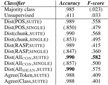
The results for the different system configurations over the four countability classes are presented in Tables 1–4, in which the highest classification accu-racy and F-score values for each class are presented in boldface. The classifier Dist(AllCON,SUITE), for
example, applies the distribution-based feature rep-resentation in a SUITE classifier configuration (i.e. it tests for binary membership in each countability class), using the concatenated feature vectors from each of the tagger, chunker and RASP.
Items of note in the results are:
Classifier Accuracy F-score
Majority class .985 (.023) Unsupervised .411 .033 Dist(POS,SUITE) .989 .558 Dist(POS,SINGLE) (.850) .479 Dist(chunk,SUITE) .990 .568 Dist(chunk,SINGLE) (.853) .495 Dist(RASP,SUITE) .989 .415 Dist(RASP,SINGLE) (.847) .360 Dist(AllCON,SUITE) .990 .582
Dist(AllCON,SINGLE) (.857) .500 Dist(AllMEAN,SUITE) .990 .575 Agree(Token,SUITE) .988 .409 Agree(Class,SUITE) .988 .401
Table 3: Basic results for plural only nouns
Classifier Accuracy F-score
Majority class .994 (.012) Unsupervised .931 .137 Dist(POS,SUITE) .997 .752 Dist(POS,SINGLE) (.850) .857 Dist(chunk,SUITE) .997 .704 Dist(chunk,SINGLE) (.853) .865
[image:6.612.95.273.241.385.2]Dist(RASP,SUITE) .997 .700 Dist(RASP,SINGLE) (.847) .798 Dist(AllCON,SUITE) .996 .723 Dist(AllCON,SINGLE) (.857) .730 Dist(AllMEAN,SUITE) .997 .710 Agree(Token,SUITE) .997 .710 Agree(Class,SUITE) .997 .695
Table 4: Basic results for bipartite nouns
• all system configurations surpass both the majority-class baseline and unsupervised clas-sifier in terms of F-score
• for all other than bipartite nouns, the SUITE classifier outperforms theSINGLE classifier in terms of F-score
• the best of the distribution-based classifiers was, without exception, superior to the best of the agreement-based classifiers
• chunk-based feature extraction generally pro-duced superior performance to POS tag-based feature extraction, which was in turn gener-ally better than RASP-based feature extraction; statistically significant differences in F-score (based on the two-tailedt-test,p < .05) were observed for both chunking and tagging over RASP for the plural only class, and chunking over RASP for the countable class
• for the SUITE classifier, system combination by either concatenation (Dist(AllCON,SUITE))
or averaging over the individual feature val-ues (Dist(AllMEAN,SUITE)) generally led to a
[image:6.612.335.517.253.395.2]0.75 0.8 0.85 0.9 0.95 1
100 1000
0.1 1 10 100
F-score
Instances/sec
No. Features (N)
rand-N(countable) best-N(countable)
best-N(uncountable)
rand-N(uncountable)
[image:7.612.76.297.69.226.2]best-N(countable) best-N(uncountable)
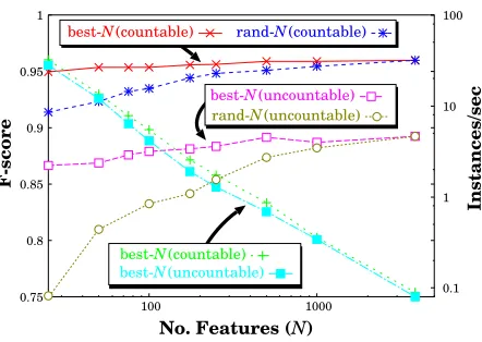
Figure 1: Effects of feature selection
and uncountable classes,4 but there was no statistical difference between these two archi-tectures for any of the 4 countability classes; for theSINGLE classifier, system combination (Dist(AllCON,SUITE)) did not lead to a signifi-cant performance gain
To evaluate the effects of feature selection, we graphed the F-score value and processing time (in instances processed per second5) over values of N from 25 to the full feature set. We targeted the Dist(AllCON,SUITE) system for evaluation (3852
features), and ran it over both the countable and un-countable classes.6 We additionally carried out ran-dom feature selection as a baseline to compare the feature selection results against. Note that thex-axis (N) and right y-axis (instances/sec) are both log-arithmic, such that the linear right-decreasing time curves are indicative of the direct proportionality be-tween the number of features and processing time. The differential in F-score for the best-N configura-tion as compared to the full feature set is statistically insignificant forN > 100for countable nouns and N >50for uncountable nouns. That is, feature se-lection facilitates a relative speed-up of around30×
without a significant drop in F-score. Comparing the results for the best-N and rand-N features, the dif-ference in F-score was statistically significant for all values ofN < 1000. The proposed method of fea-ture selection thus allows us to maintain the full clas-sification potential of the feature set while enabling
4
No significant performance difference was observed for:
Dist(ChunkMEAN,SUITE) vs. Dist(All∗,SUITE) for countable
nouns, and Dist(POSCON,SUITE) vs. Dist(AllCON,SUITE) for
uncountable nouns.
5
As evaluated on an AMD Athlon 2100+CPU with 3GB of memory.
6
We focus exclusively on countable and uncountable nouns here and in the remainder of supplementary evaluation as these are by far the most populous countability classes.
Feature COUNTABLE UNCOUNTABLE
space Acc F-score Acc F-score
All features .937 .959 .954 .895 Best-200 .934 .956 .949 .884 Binary .904∗ .931∗ .930∗ .833∗ Corpus freq .929 .954 .952 .889 Word freq .933 .956 .954 .896 Feature freq .928 .952∗ .934∗ .869∗
Table 5: Results for restricted feature sets
a speedup greater than an order of magnitude, po-tentially making the difference in practical utility for the proposed method.
To determine the relative impact of the com-ponent feature values on the performance of the distribution-based feature representation, we used the Dist(AllMEAN,SUITE) configuration to build: (a)
a classifier using a single binary value for each unit feature, based on simple corpus occurrence
(Bi-nary); and (b) 3 separate classifiers based on each of
thecorpfreq,wordfreq andfeatfreq features values only (without the 2D feature cluster totals). In each case, the total number of feature values is 206.
The results for each of these classifiers over countable and uncountable nouns are pre-sented in Table 5, as compared to the basic
Dist(AllMEAN,SUITE) classifier with all 1,284
features (All features) and also the best-200 features (Best-200). Results which differ from those for
All features to a level of statistical significance are
asterisked. The binary classifiers performed signif-icantly worse than All features for both countable and uncountable nouns, underlining the utility of the distribution-based feature representation. wordfreq is marginally superior to corpfreq as a standalone feature representation, and both of these were on the whole slightly below the full feature set in performance (although no significant difference was observed). featfreq performed slightly worse again, significantly below the level of the full feature set. Results for the best-200 classifier were marginally higher than those for each of the individual feature representations in the case of the countable class, but marginally below the results for corpfreq and
wordfreq in the case of the uncountable class. The differences here are not statistically significant, and additional evaluation is required to determine the relative success of feature selection over simply usingwordfreq values, for example.
6 Discussion
[image:7.612.321.528.72.153.2]cor-pora. Bond and Vatikiotis-Bateson (2002) deter-mine a noun’s countability preferences—as de-fined in a 5-way classification—from its se-mantic class in the ALT-J/E lexicon, and show that semantics predicts countability 78% of the time. O’Hara et al. (2003) implemented a sim-ilar approach using the much larger Cyc on-tology and achieved 89.5% accuracy, mapping onto the 2 classes of countable and uncount-able. Schwartz (2002) learned noun countabilities by looking at determiner occurrence in singular noun chunks and was able to tag 11.7% of BNC noun tokens as countable and 39.5% as uncountable, achieving a noun type agreement of 88% and 44%, respectively, with the ALT-J/E lexicon. Our results compare favourably with each of these.
In a separate evaluation, we took the best-performing classifier (Dist(AllCON,SUITE)) and ran it over open data, using best-500 feature selection (Baldwin and Bond, 2003). The output of the classifier was evaluated relative to hand-annotated data, and the level of agreement found to be around 92.4%, which is approximately equivalent to the agreement betweenCOMLEXandALT-J/Eof 93.8%. In conclusion, we have presented a plethora of learning techniques for deep lexical acquisition from corpus data, and applied each to the task of classify-ing English nouns for countability. We specifically compared two feature representations, based on rel-ative feature occurrence and token-level classifica-tion, and two basic classifier architectures, using a suite of binary classifiers and a single multi-class classifier. We also analysed the effects of comb-ing the output of multiple processors, and pre-sented a simple feature selection method. Overall, the best results were obtained using a distribution-based suite of binary classifiers combining the out-put of multiple pre-processors.
Acknowledgements
This material is based upon work supported by the National Science Foundation under Grant No. BCS-0094638 and also the Research Collaboration between NTT Communication Sci-ence Laboratories, Nippon Telegraph and Telephone Corpora-tion and CSLI, Stanford University. We would like to thank Leonoor van der Beek, Slaven Bilac, Ann Copestake, Ivan Sag and the three anonymous reviewers for their valuable input on this research, and John Carroll for providing access to RASP.
References
Timothy Baldwin and Francis Bond. 2003. Learning the count-ability of English nouns from corpus data. In Proc. of the
41st Annual Meeting of the ACL, Sapporo, Japan. (to
ap-pear).
Francis Bond and Caitlin Vatikiotis-Bateson. 2002. Using an ontology to determine English countability. In Proc. of the
19th International Conference on Computational Linguistics (COLING 2002), Taipei, Taiwan.
Ted Briscoe and John Carroll. 2002a. High precision extraction of grammatical relations. In Proc. of the 19th International
Conference on Computational Linguistics (COLING 2002),
pages 134–140, Taipei, Taiwan.
Ted Briscoe and John Carroll. 2002b. Robust accurate sta-tistical annotation of general text. In Proc. of the 3rd
In-ternational Conference on Language Resources and Evalu-ation (LREC 2002), pages 1499–1504, Las Palmas, Canary
Islands.
Lou Burnard. 2000. User Reference Guide for the British
Na-tional Corpus. Technical report, Oxford University
Comput-ing Services.
Jean Carletta. 1996. Assessing agreement on classifica-tion tasks: the kappa statistic. Computaclassifica-tional Linguistics, 22(2):249–254.
Walter Daelemans, Jakub Zavrel, Ko van der Sloot, and An-tal van den Bosch. 2002. TiMBL: Tilburg memory based
learner, version 4.2, reference guide. ILK technical report
02-01.
Ralph Grishman, Catherine Macleod, and Adam Myers, 1998.
COMLEX Syntax Reference Manual. Proteus Project, NYU.
(http://nlp.cs.nyu.edu/comlex/refman.ps). Satoru Ikehara, Satoshi Shirai, Akio Yokoo, and Hiromi
Nakaiwa. 1991. Toward an MT system without pre-editing – effects of new methods in ALT-J/E–. In Proc. of the Third
Machine Translation Summit (MT Summit III), pages 101–
106, Washington DC, USA.
Huan Liu and Hiroshi Motoda. 1988. Feature Extraction,
Con-struction and Selection: A Data Mining Perspective. Kluwer
Academic Publishers.
Guido Minnen, John Carroll, and Darren Pearce. 2001. Ap-plied morphological processing of English. Natural
Lan-guage Engineering, 7(3):207–23.
Grace Ngai and Radu Florian. 2001. Transformation-based learning in the fast lane. In Proc. of the 2nd Annual Meeting
of the North American Chapter of Association for Compu-tational Linguistics (NAACL2001), pages 40–7, Pittsburgh,
USA.
Tom O’Hara, Nancy Salay, Michael Witbrock, Dave Schnei-der, Bjoern Aldag, Stefano Bertolo, Kathy Panton, Fritz Lehmann, Matt Smith, David Baxter, Jon Curtis, and Peter Wagner. 2003. Inducing criteria for mass noun lexical map-pings using the Cyc KB and its extension to WordNet. In
Proc. of the Fifth International Workshop on Computational Semantics (IWCS-5), Tilburg, the Netherlands.
Lane O.B. Schwartz. 2002. Corpus-based acquisition of head
noun countability features. Master’s thesis, Cambridge
Uni-versity, Cambridge, UK.
Erik F. Tjong Kim Sang and Sabine Buchholz. 2000. Introduc-tion to the CoNLL-2000 shared task: Chunking. In Proc.
of the 4th Conference on Computational Natural Language Learning (CoNLL-2000), Lisbon, Portugal.
Allan P. White and Wei Zhong Liu. 1994. Bias in information-based measures in decision tree induction. Machine