A u t o m a t e d Construction of Database Interfaces: Integrating
Statistical and Relational Learning for Semantic Parsing
L a p p o o n R . T a n g a n d R a y m o n d J . M o o n e y D e p a r t m e n t of C o m p u t e r Sciences
University of Texas at A u s t i n Austin, T X 78712-1188
{rupert, mooney}@cs, utexas, edu
A b s t r a c t
The development of natural language inter- faces (NLI's) for databases has been a chal- lenging problem in natural language process- ing (NLP) since the 1970's. The need for NLI's has become more pronounced due to the widespread access to complex databases now available through the Internet. A challenging problem for empirical NLP is the automated acquisition of NLI's from training examples. We present a method for integrating statisti- cal and relational learning techniques for this task which exploits the strength of both ap- proaches. Experimental results from three dif- ferent domains suggest that such an approach is more robust t h a n a previous purely logic- based approach.
1 I n t r o d u c t i o n
We use the term
semantic parsing
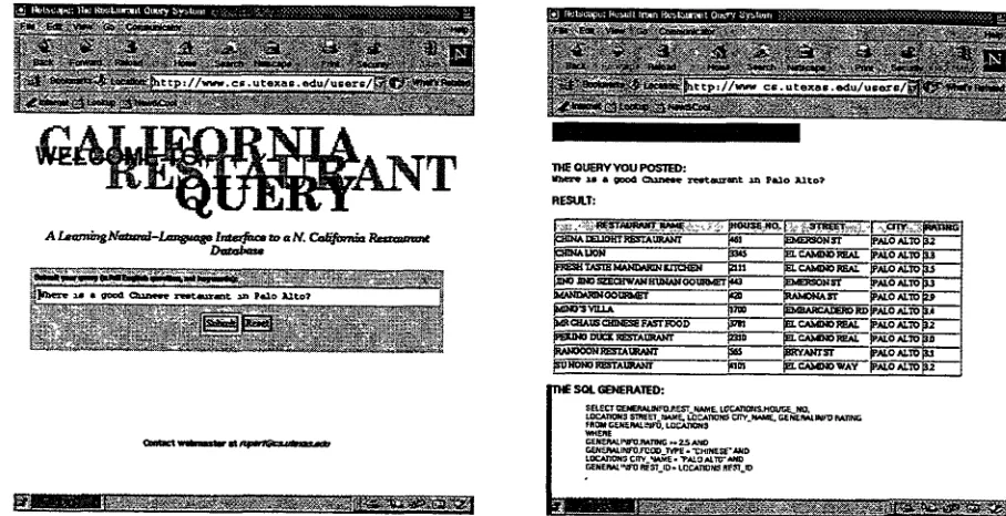
to refer to the process of mapping a natural language sentence to a structured meaning representa- tion. One interesting application of semantic parsing is building natural language interfaces for online databases. The need for such appli- cations is growing since when information is delivered through the Internet, most users do not know the underlying database access lan- guage. An example of such an interface that we have developed is shown in Figure 1.Traditional
(rationalist)
approaches to con- structing database interfaces require an ex- pert to hand-craft an appropriate semantic parser (Woods, 1970; Hendrix et al., 1978). However, such hand-crafted parsers are time consllming to develop and suffer from prob- lems with robustness and incompleteness even for domain specific applications. Neverthe- less, very little research in empirical NLPhas
explored the task of automatically acquiring
such interfaces from annotated training ex- amples. The only exceptions of which we are aware axe a statistical approach to map-ping airline-information queries into SQL pre- sented in (Miller et al., 1996), a probabilistic decision-tree method for the same task de- scribed in (Kuhn and De Mori, 1995), and an approach using relational learning (a.k.a.
inductive logic programming,
ILP) to learn a logic-based semantic parser described in (Zelle and Mooney, 1996).The existing empirical systems for this task employ either a purely logical or purely sta- tistical approach. The former uses a deter- ministic parser, which can suffer from some of the same robustness problems as rational- ist methods. The latter constructs a prob- abilistic grammar, which requires supplying a sytactic parse tree as well as a semantic representation for each training sentence, and requires hand-crafting a small set of contex- tual features on which to condition the pa- rameters of the model. Combining relational and statistical approaches can overcome the need to supply parse-trees and hand-crafted features while retaining the robustness of sta- tistical parsing. The current work is based on the CHILL logic-based parser-acquisition framework (Zelle and Mooney, 1996), retain- ing access to the complete parse state for mak- ing decisions, but building a probabilistic re- lational model that allows for statistical pars- ing-
2 O v e r v i e w o f t h e A p p r o a c h
This section reviews our overall approach using an interface developed for a U.S. Geography database (Geoquery) as a sample application (ZeUe and Mooney, 1996) which is available on the Web (see
hl:tp://gvg,
c s . u t e z a s ,edu/users/n~./geo .html).
2.1 S e m a n t i c R e p r e s e n t a t i o n
D a m b a ~
QUERY YOU PO~TED:
all a goo~ ~ z ~ c a L ~ ~m ~ o ~.t~o'P RE~UI.T:
~ o o a ~ e ~ I,~ p . ~ . , . ~ r ~ , ~ o ~ o ~ J ~u~,,o~ ",,~u.,. p~o ~ . ~ . , , ¢ B o ~ ~,.~.o ,~.~o ~.~ I
a ~ o o o ~ z ~ u ~ r ~ ~ ~ r r ~ r ~,~o~.~o ~ I
THE SOL GENERATED:
~n0~t ~ . K ~ t ~Fo, LOCAnONS C ~ * t l ~ r O J t ~ ~ Z3 AgO
Figure 1: Screenshots of a Learned Web-based NL Database Interface
automatically into SQL (see Figure 1). We explain the features of the Geoquery repre- sentation language through a sample query:
Input: "W'hat is the largest city in Texas?"
Quc~'y: a nswer(C,largest(C,(city(C),loc(C,S),
const (S,stateid (texas))))).
Objects are represented as logical terms and are typed with a semantic category using logical functions applied to possibly ambigu- ous English constants (e.g.
stateid(Mississippi),
riverid(Mississippi)).
Relationships between ob- jects are expressed using predicates; for in- stance, Ioc(X,Y) states that X is located in Y. We also need to handle quantifiers such as 'largest'. We represent these using meta-predicates for which at least one argument is a
conjunction ofliterals. For example, largest(X, Goal) states that the object X satisfies Goal and is the largest object that does so, using the appropriate measure of size for objects of its type (e.g. area for states, population for cities). Finally, an nn.qpeci~ed object required as an argument to a predicate can appear else- where in the sentence, requiring the use of the predicate const(X,C) to bind the variable X to the constant C. S o m e other database queries
(or training examples) for the U.S. Geography domain are shown below:
What is the capital of Texas?
a nswer(C,(ca pital(C,S),const(S,stateid (texas)))).
What state has the most rivers running through it? a nswer(S,most (S,R,(state(S),rlver(R),traverse(R,S)))).
2.2 P a r s i n g Actions
Our semantic parser employs a shift-reduce architecture that maintains a stack of pre- viously built semantic constituents and a buffer of remaining words in the input. The parsing actions are automatically generated from templates given the training data. The templates are INTRODUCE, COREF_VABS, DROP_CON J, LIFT_CON J, and SttIFT. IN- TRODUCE pushes a predicate onto the stack based on a word appearing in the input and information about its possible meanings in the lexicon. C O R E F _ V A R S binds two argu- ments of two different predicates on the stack. D R O P _ C O N J (or L I F T _ C O N J) takes a pred- icate on the stack and puts it into one of the arguments of a meta-predicate on the stack. S H I F T simply pushes a word from the input buffer onto the stack. T h e parsing actions are tried in exactly this order. T h e parser also requires a lexicon to map phrases in the in- put into specific predicates, this lexicon can also be learned automatically from the train- ing data (Thompson and Mooney, 1999).
[image:2.596.108.562.85.318.2]here. Interrogatives like "what" m a y be m a p p e d to predicates in t h e lexicon if neces- sary. The parser begins with an initial stack a n d a buffer holding the i n p u t sentence. Each predicate on the parse stack has an attached buffer to hold t h e context in which it was introduced; words from t h e i n p u t sentence are shifted onto this buffer during parsing. The initial parse state is shown below:
Parse Stack:
[answer(_,_):O]
Input Buffer:
[what,is,the,ca pital,of,texas,?]
Since the first three words in the i n p u t buffer do not m a p to any predicates, three SHIFT actions are performed. T h e next is an I N T R O D U C E as 'capital' is at t h e head of the input buffer:
Parse Stack:
[capital(_,_): O, answer(_,_):[the,is,what]]
Input Buffer: [capital,of,texas,?]
The next action is a C O R E F _ V A R S that binds the first argument of
capital(_,_)
with the first argument of answer(_,_).Parse Stack: [capital(C,_): O, answer(C,_):[the,is,what]]
Input Buffer:
[capital,of,texas,?]
The next sequence of steps axe two SHIFT's, an I N T R O D U C E , and then a C O R . E F _ V A R S :
Parse Stack: [const(S,stateid(texas)): 0' ca pital(C,S):[of, ca pital], answer(C,_):[the,is,what~
Input Buffer: [texas,?]
T h e last four steps are two DROP_CONJ's followed by two SHIFT's:
Parse Stack:
[answer(C, (capital(C,S),
const(S,stateld(texas)))): [?,texas,of, ca pital,the,is,what]]Input Buffer: I]
This is the final state a n d t h e logical query is extracted from t h e stack.
2.3 Learning Control Rules
T h e initially constructed parser has no con- straints on w h e n to apply actions, and is therefore overly general and generates n11rner- ous spurious parses. Positive and negative ex- amples are collected for each action by parsing
each tralnlng example and recordlng t h e parse states encountered. Parse states to which an action should be applied (i.e. the action leads to building t h e correct semantic representa- tion) are labeled positive examples for t h a t action. Otherwise, a parse state is labeled a
negative example for an action if it is a posi- tive example for another action below t h e cur- rent one in t h e ordered list of actions. Control conditions which decide t h e correct action for a given parse state axe learned for each action from these positive a n d negative examples.
The initial CHILL system used ILP (Lavrac and Dzeroski, 1994) to learn Prolog control rules and employed deterministic parsing, us- ing the learned rules to decide the appropriate parse action for each state. T h e current ap- proach learns a model for estimating t h e prob-
ability t h a t each action should be applied to
a given state, and employs statistical parsing (Manning a n d Schiitze, 1999) to try to find the overall most probable parse, using beam search to control the complexity. T h e advan- tage of ILP is that it can perform induction over the logical description of the complete parse state without t h e need to pre-engineer a fixed set of features (which vary greatly from one domain to another) t h a t are relevant to
making decisions. W e maintain this advan- tage by using ILP to learn a committee of hypotheses, a n d basing probability estimates on a weighted vote of t h e m (Ali and Pazzani,
1996). W e believe that using such a proba- bilistic relational model (Getoor and Jensen, 2000) combines the advantages of frameworks based on first-order logic and those based on standard statistical techniques.
3 T h e TABULATE I L P
M e t h o d
This section discusses t h e I L P m e t h o d used to build a committee of logical control hypothe- ses for each action.
3.1
The
B a s i c TABULATEAlgorithm
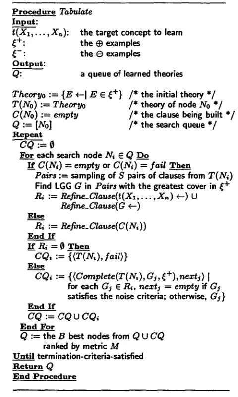
Most I L P m e t h o d s use a set-covering m e t h o d to learn one clause (rule) at a time a n d con- struct clauses using either a strictly top-down (general to specific) or b o t t o m - u p (specific to general) search t h r o u g h t h e space of possi- ble rules (Lavrac a n d Dzeroski, 1994). TAB- ULATE, 1 on the other hand, employs b o t h b o t t o m - u p and top-down m e t h o d s to con- struct potential clauses a n d searches t h r o u g h the hypothesis space of complete logic pro- grams (i.e. sets of clauses called theories). It uses b e a m search to find a set of alternative hypotheses guided by a theory evaluation met- ric discussed below. T h e search starts with
Procedure Tabulate Input:
t ( X , , . . . , X n ) : the target concept to learn
~+: the (B examples
~ - : the (9 examples
Output:
Q: a queue of learned theories
Theoryo := {E '¢'-I E E ~+} /* the initial theory */
T(No) := Theoryo /* theory of node No */
C(No) := empty /* the clause being built */
Q := [No] /* the search queue */
R e p e a t
CO ¢
Fo_._X each search node Ni E Q D__q
C(Ni) = empty or C(Ni) = fail T h e n
Pairs := sampling of S pairs of clauses from T(N~)
Find LGG G in Pairs with the greatest cover in ~+ Ri := Refine_Clause(t(X1,... ,Xn) +-) U
Refine_Clause( G ~--) Else
R4 := Reflne_Clause(C(Ni))
E n d I f
I f Ri ---- ¢ T h e n
CQ,
:= {(T(N,),fail)}
ElseCQi
:={(Coraplete(T(N,),
Gj,~+),
neztj) [
for each G~ E ,,~, next~ = empty if Gjsatisfies the noise criteria; otherwise, G$} E n d I f
C Q : = C Q u CQ~
End For
Q := the B best nodes from Q U CQ
ranked by metric M U n t i l terminatlon-criteria-satisfied
R e t u r n Q
E n d P r o c e d u r e
Figure 2: T h e TABULATE algorithm
t h e most specific hypothesis (the set of posi- tive examples each represented as a separate clause). Each iteration of the loop a t t e m p t s to refine each of t h e hypotheses in the current search queue. T h e r e are two cases in each it- eration: 1) an existing clause in a theory is refined or 2) a new clause is begun. Clauses are learned using b o t h top-down specialiT.~- tion using a m e t h o d similar to FOIL (Quin- lan, 1990) and b o t t o m - u p generalization using Least General Generalizations (LGG's). Ad- vantages of combining b o t h I L P approaches were explored in CHILLIN (ZeUe and Mooney, 1994), an ILP m e t h o d which motivated t h e design of TABULATE. A n outline of t h e TAB- ULATE algorithm is given in Figure 2.
A noise-handling criterion is used to de-
cide when an individual clause in a hypoth- esis is sufficiently accurate to be permanently
retained. There are three possible outcomes in a refinement: 1) t h e current clause satisfies the noise-handling criterion a n d is simply re-
turned (nextj is set to empty), 2) t h e current
clause does not satisfy t h e noise-handling cri- teria a n d all possible refinements are returned
(neztj is set to t h e refined clause), a n d 3)
t h e current clause does n o t satisfy t h e noise- handling criterion b u t there are no further re- finements (neztj is set to fai O. If t h e refine- ment is a new clause, clauses in t h e current theory subs-reed by it are removed. Oth- erwise, it is a specialization of an existing clause. Positive examples t h a t are n o t cov- ered by t h e resulting theory, due to special- izing t h e clause, are a d d e d back into theory as individual clauses. Hence, t h e theory is al- ways maintained complete (i.e. covering all positive examples). These final steps are per- formed in the Complete procedure.
The termination criterion checks for two conditions. T h e first is satisfied if t h e next search queue does not improve t h e s u m of t h e metric score over all hypotheses in t h e queue. Second, there is no clause currently being built for each theory in t h e search queue and t h e last finished clause of each theory sat- isfies t h e noise-handling criterion. Finally, a committee of hypotheses found by t h e algo- rithm is returned.
3 . 2 C o m p r e s s i o n a n d A c c u r a c y
T h e goal of t h e search is to find accurate a n d yet simple hypotheses. We measure accu- racy using the m-estimate (Cestnik, 1990), a smoothed measure of accuracy on t h e training d a t a which in t h e case of a two-class problem is defined as:
accuracy(H) = s + m . p + (1)
n ,-I- rrt
where s is t h e n - t u b e r of positive examples covered by t h e hypothesis H , n is t h e total n u m b e r of examples covered, p+ is t h e prior probability of t h e class (9, a n d m is a smooth- ing parameter.
We measure theory complexity using a met- ric slmi]ar to t h a t introduced in (Muggleton a n d Buntine, 1988). T h e size of a Clause hav-
ing a Head and a Body is defined as follows
( t s = " t e r m size" a n d a r = " a r i t y ' ) :
[image:4.596.96.336.89.489.2]I 1
T is a variable
ts(T) = 2 r ~,, ¢ o ~ t
2 +
ts(argi(T))
(3)
T h e size of a clause is roughly t h e n,,mber of variables, constants, or predicate symbols it contains. T h e size of a t h e o r y is t h e s u m of the sizes of its clauses. T h e m e t r i c M ( H ) used as t h e search heuristic is defined as:M ( H ) = accuracy(H) + C
log 2 size(H) (4)
where C is a constant used to control t h e rel- ative weight of accuracy vs. complexity. We ass~,me t h a t t h e most general hypothesis is as good as the most specific hypothesis; thus, C is determined to be:
C
= EbSt --EtSb
(5)& - &
where Et, Eb are t h e accuracy estimates of t h e most general and most specific hypotheses re- spectively, and St, Sb are their sizes.
3.3 N o i s e H a n d l i n g
A clause needs no f u r t h e r refinement when it meets the following criterion (as in RIPPER (Cohen, 1995)):
P
-.__.2_ >
(6)
p + n
where p is t h e n u m b e r of positive examples covered by t h e clause, n is t h e n u m b e r of neg- ative examples covered a n d - 1 < / ~ _< 1 is a parameter. T h e value of ~ is decreased when- ever t h e s u m of t h e m e t r i c over t h e hypotheses in t h e queue does not improve a l t h o u g h some of t h e m still have ,nflni~hed or failed clauses.
4
Statistical Semantic Parsing
4.1 T h e P a r s i n g M o d e lA parser is a relation Parser C_ Sentences x
Queries where Sentences and Queries are
t h e sets of n a t u r a l language sentences a n d database queries respectively. Given a sen- tence I • Sentences, t h e set Q(1) = {q •
Queries I (l, q) • Parser} is t h e set of queries
t h a t are correct interpretations of I.
A parse state consists of a stack of lexical-
ized predicates a n d a list of words from t h e
i n p u t sentence. S is t h e set of states reach- able by the parser. Suppose our learned parser has n different parsing actions, t h e i t h ac- tion a / i s a function a/(s) : I S i -+ OSi where
ISi G S is t h e set of states to which t h e ac-
tion is applicable a n d OSi C_ S is t h e set of states constructed by t h e action. T h e function
ao(l) : Sentences ~ IniS m a p s each sentence l
to a corresponding unique initial parse state in In/S C_ S. A state is called afinalstate if there exists no parsing action applicable to it. T h e
partial function a,+l(s) : FS ~ Queries is
defined as t h e action t h a t retrieves t h e query from the final state s 6 FS C S if one exists. Some final states m a y not "contain" a query (e.g. w h e n t h e parse stack contain.q predicates with u n b o u n d ~rariables) a n d therefore it is a partial function. W h e n t h e parser meets such a final state, it reports a failure.
A path is a finite sequence of parsing ac-
tions. Given a sentence 1, a good s t a t e s is one such t h a t there exists a p a t h from it to a query q 6 Q(1). Otherwise, it is a bad state. T h e set of parse states can b e uniquely divided into t h e set of good states a n d t h e set of b a d states given l a n d Parser. S + and S - are t h e sets of good a n d bad states respectively.
Given a sentence l, t h e goal is to construct t h e query ~ such t h a t
= argmqaX P(q • Q(l) [ l ~ q) (7)
where I ~ q means a p a t h exists from l to q. Now, we need to e s t i m a t e P(q • Q(1) I l =-~
q). First, we notice that:
P(q • Q(1) [l =~. q) ---- (8)
P ( s • FS + I I ~ s a n d an+l(S) ---- q)
where F S + = FS N S +. For notational con- venience we drop t h e conditions a n d d e n o t e t h e above probabilities as P(q • Q(l)) and
P(s • FS +) respectively, assuming these con-
ditions in t h e following discussion. T h e equa- tion states t h a t t h e probability t h a t a given query is a correct m e a n i n g for I is t h e s a m e as t h e probability t h a t t h e final state (reached by parsing l) is a good state. We need to de- termine in general t h e probability of having a good resulting parse state. Given a n y parse state s i at t h e j t h step o f parsing a n d a n ac- tion ai such t h a t si+1 = a/(sj), we have:
PCsi+1 •
(9)
pCsj+l e o & +
I
•
x&+)pCs • x& +) +
P ( S i + l • OSi +
I
sj
¢ISi+)P(sj
¢~ISi
+)
where IS~ =
ISi N S + and OS~ = OS~ N S +.
parse state from a bad one, t h e second t e r m is zero. Now, we are ready to derive P(q •
Q(l)). Suppose q = an+l(Sm), we have:
P(q 6 Q(l)) (10)
= P ( s ~ • F ~ )
...
= P(s,n • F S +
l
sm-1 •/St,_a)...
P(s~ • OS~_,
I sj-1 •
I s ~ _ , ) . . .
P(s2 • Ob~,
Is1 •
IS~, ) P ( ' I • IS~,)where ak denotes t h e index of which action is applied at t h e k t h step. We assume t h a t
= P ( s l • I~aa) ~ 0 (which m a y not be t r u e
in general). Now, we have
m - - I
P(q 6 Q(l))
= 7 I I P(sj+I •
O ~
l sj •
IS~-3).i=l
(11)
Next we describe how we estimate the proba- b i l i ~ of t h e goodness of each action in a given
state (P(~(s) • o $ I s • I ~ ) ) . We n ~
not estimate7
since its value does not affect t h e outcome of equation (7).4 . 2 E s t i m a t i n g P r o b a b i l i t i e s f o r P a r s i n g A c t i o n s
T h e committee of hypotheses learned by TAB- ULATE is u s e d t o e s t i m a t e t h e probability t h a t a particular action is a good one to apply to a given parse state. Some hypotheses are more
"important" t h a n others in t h e sense t h a t they carry more weight in t h e decision. A weight- ing parameter is also included to lower t h e probability estimate of actions t h a t appear fm'ther down the decision list. For actions ai where 1 < i < n - 1:
P(ai(s) • o ~
Is •
Is7-) =
.po,(i)-I ~ AkP(~Cs) 6 0 b ~ ~ I h~)
hk~H~
(12)
where s is a given parse state, pos(i) is t h e position of t h e action ai in t h e list of ac- tions applicable to state s, Ak a n d 0 < /~ < 1 are weighting parameters, z Hi is the set of hypotheses learned for t h e action ai, a n d ~ k A~ = 1.
To estimate t h e probability for t h e last ac- tion an, we devise a simple test t h a t checks if t h e m a x i m u m of t h e set A(s) of proba- bility estimates for t h e subset o f the actions
2p is set t o 0.95 for all the experiments performed.
{ a l , . . . , a n - l } applicable to s is less t h a n or equal to a threshold a . If A(s) is empty, we assume t h e maxlrn,,rn is zero. More precisely,
PCa.Cs) • o s ~ Is • xs~) =
{ ,c..(,)~os~) if maxCACs)) <
~(,~IS~)
0 otherwise
(13)
where a is t h e threshold, 3 c(an(s) • Ob~) is
the count of t h e n u m b e r of good states pro- duced by t h e last action, a n d c(s • IS~) is the count of t h e n u m b e r of good states to which the last action is applicable.
Now, let's
discuss
how P(ai(s) • OS~ ~ I hk)and Ak are estimated. If hk ~ s (i.e. hk covers s), we have
PCai(s) • o ~
I hk) =
pc + O " ncPc -t- nc
(14)
where Pc a n d ne are t h e n u m b e r of positive and negative examples covered by hk respec- tively. Otherwise, if h~ ~= s (i.e. hk does not cover s), we have
PCai(s) • OS 7"
I hk)
-- p" + 8 . n , ,Pu + n u
(15)
where Pu and nu are t h e n,,rnber of positive and negative examples rejected by hk respec- tively. /9 is t h e probability that a negative example is mislabelled a n d its value can be estimated given # (in equation (6)) a n d t h e total nnrnber of positive a n d negative exam- ples.One could use a variety of linear combina- tion m e t h o d s to estimate t h e weights Ak (e.g. Bayesian combination (Buntine, 1990)). How- ever, we have taken a simple approach a n d weighted hypotheses based on their relative simplicity:
size(hk) -1
Ak = ~.lHd size(hi)_1" (16) z-d=l
4.3 S e a r c h i n g f o r a P a r s e
To find t h e most probably correct parse, t h e parser employs a b e a m search. At each step, the parser finds all of t h e parsing actions ap- plicable to each parse state on the queue a n d calculates t h e probability of goodness of each of t h e m using equations (12) a n d (13). It t h e n
computes the probability t h a t t h e resulting state of each possible action is a good state using equation (11), sorts t h e queue of possi- ble next states accordingly, a n d keeps t h e best B options. T h e parser stops when a complete parse is found on the top of t h e parse queue or a failure is reported.
5 E x p e r i m e n t a l R e s u l t s
5.1 T h e D o m a i n s
Three different domains are used to demon- strate the performance of t h e new approach. T h e first is the U.S. Geography domain. T h e database contains about 800 facts a b o u t U.S. states like population, area, capital city, neighboring states, major rivers, m a j o r cities, and so on. A hand-crafted parser, GEOBASE was previously constructed for this d o m a i n as a demo product for Turbo Prolog. T h e second application is the restaurant query system il- lustrated in Figure 1. T h e database contains information about thousands of restaurants in Northern California, including t h e name of the restaurant, its location, its specialty, and a guide-book rating. The t h i r d domain consists of a set of 300 computer-related jobs automat- ically extracted from postings to t h e U S E N E T newsgroup a u s t i n . j o b s . T h e database con- talus the following information: t h e job title, the company, the recruiter, t h e location, t h e salary, the languages and platforms used, a n d required or desired years of experience a n d de- grees.
5.2 E x p e r i m e n t a l D e s i g n
T h e geography corpus contains 560 questions. Approximately 100 of these were collected from a log of questions s u b m i t t e d to the web site and the rest were collected in studies in- volving students in undergraduate classes at our university. We also included results for t h e subset of 250 sentences originally used in t h e experiments reported in (Zelle a n d Mooney, 1996). The remaining questions were specif- icaUy collected to be more complex t h a n t h e original 250, and generally require one or more meta-predicates. The restaurant corpus con- taln~ 250 questions automatically generated from a hand-built g r a m m a r C o n s t r u c t e d t o re- flect typical queries in this domain. T h e job corpus contains 400 questions automatically generated in a similar fashion. T h e beam w i d t h for TABULATE was set~ to five for all t h e domains. T h e deterministic parser used only t h e best hypothesis found. T h e experiments
were conducted using 10-fold cross validation. For each domain, the average recall (a.k.a. accuracy) a n d precision of t h e parser on dis- joint test d a t a are reported where:
of correct queries produced
R e c a l l =
of test sentences
P r e c i s i o n = # of correct queries produced
# of complete parses produced"
A complete parse is one which contains an ex- ecutable query (which could be incorrect). A query is considered correct if it produces the same answer set as t h e gold-standard query supplied with the corpus.
5.3 R e s u l t s
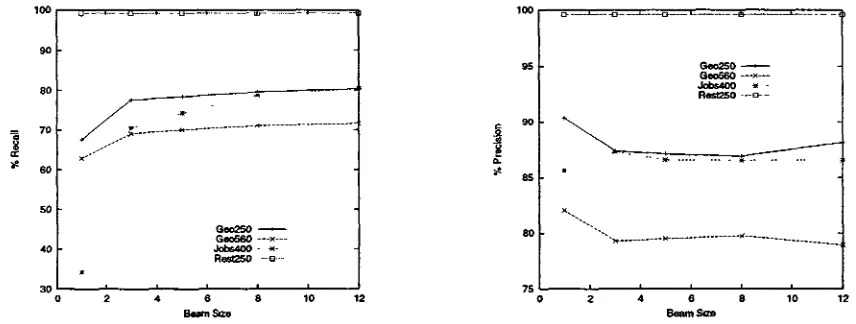
T h e results are presented in Table 1 and Fig- ure 3. By switching from deterministic to probabilistic parsing, t h e system increased the number of correct queries it produced. Re- call increases almost monotonically with pars- ing beam width in most of the domains. I_m- provement is most apparent in the Jobs do-
maln where probabilistic parsing signiBcantly outperformed t h e deterministic system (80% vs 68%). However, using a b e a m width of one (and thus the probabilistic parser picks only the best action) results in worse perfor- mance t h a n using t h e original purely logic- based determlni~tic parser. This suggests t h a t the probability esitmates could be improved since overall they are not indicating t h e sin- gle best action as well as a non-probabilistic approach. Precision of t h e system decreased with b e a m width, b u t not signi~cantly except for the larger Geography corpus. Since t h e system conducts a more extensive search for a complete parse, it risks increasing the num- ber of incorrect as well as correct parses. T h e importance of recall vs. precision depends on t h e relative cost of providing an incorrect an- swer versus no answer at all. Individual ap- plications may require emphasizing one or the other.
Parsers \ Corpora Geo250 Geo560 Jobs400 Rest250 Prob-Parser(12)
Prob-Parser(8) Prob-Parser(5) Prob-Parser(3) Prob-Parser(1) TABULATE Original CHILL Hand-Built Parser
R P
80.40 88.16 79.60 86.90 78.40 87.11 77.60 87.39 67.60 90.37 75.60 92.65 68.50 97.65 56.00 96.40
R P
71.61 78.94 71.07 79.76 70.00 79.51 69.11 79.30 62.86 82.05 69.29 89.81
I~ P 80.50 86.56 78.75 86.54 74.25 86.59 70.50 87.31 34.25 85.63 68.50 87.54
R P
99.20 99.60 99.20 99.60 99.20 99.60 99.20 99.60 99.20 99.60 99.20 99.60
Table 1: Results For All Domains: R = % Recall and P = % Precision. Prob-Parser(B) is the probabilistic parser using a beam width of B. TABULATE is CHILL using the TABULATE induction algorithm with determ;nistic parsing.
1 0 0 ~.
9O
8 0
7 0
60
5 0
4 0
3 0
0
G e o 2 5 0 ,
G e o 5 6 0 - - - × - - -
J o b s 4 0 0 - ~ *
R e s t 5 0 - ~ -
100
95
90
85
80
i i i i / 7 5
2 4 6 8 lO 1 2
B ~ n ,~Ze
Geo250 , Geo560 - - - x - - - Job¢,400 ~ - Rest250 - - - c - -
~ - ~ ...
x , , . . .
i i i /
2 4 6 8 10 12
Seam S ¢ ~
Figure 3: The recall and precision of the parser using various beam widths in the different domains
While there was an overall improvement in recall using the new approach, its performance varied signiGcantly from dom~;~ to domain. As a result, the recall did not always improve dramatically by using a larger beam width. Domain factors possibly affecting the perfor- mance are the quality of the lexicon, the rel- ative amount of d a t a available for calculat- ing probability estimates, and the problem of '~parser incompleteness" with respect to the test d a t a (i.e. there is not a p a t h from a sen- tence to a correct query which happens when '7 = 0). The performance of all systems were basically equivalent in the restaurant domain, where they were near perfect in both recall and precision. This is because this corpus is relatively easier given the restricted range of possible questions due to the limited informa- tion available about each restaurant. The sys- tems achieved > 90% in recall and precision given only roughly 30% of the training data in this domain. Finally, GEOBASE p e r f o m e d
the worst on the original geography queries, since it is difficult to hand-crat~ a parser that handles a sn~cient variety of questions.
6 C o n c l u s i o n
A probabilistic framework for semantic shift- reduce parsing was presented. A new ILP learning system was also introduced which learns multiple hypotheses. These two tech- niques were integrated to learn semantic parsers for building NLI's to on|ine databases. Experimental results were presented that demonstrate t h a t such a n approach outper- forms a purely logical approach in terms of the accuracy of the learned parser.
7 A c k ~ n o w l e d g e m e n t s
[image:8.596.151.520.85.215.2] [image:8.596.124.552.280.442.2]R e f e r e n c e s
K. Ali and M. Pazzani. 1996. Error reduction through learning multiple descriptions. Ma-
chine Learning Journal, 24:3:100--132.
W. Buntine. 1990. A theory of learning classifica-
tion rules. Ph.D. thesis, University of Technol-
ogy, Sydney, Australia.
B. Cestnik. 1990. Estimating probabilities: A cru- cial task in machine learning. In Proceedings of the Ninth European Conference on Artificial In-
teUigence, pages 147-149, Stockholm, Sweden.
W. W. Cohen. 1995. Fast effective rule induc- tion. In Proceedings of the Twelfth Interna- tional Conference on Machine Learning, pages
115-123.
L. Getoor and D. Jensen, editors. 2000. Papers from the AAA1 Workshop on Learning Statis-
tical Models from Relational Data, Austin, TX.
AAAI Press.
G. G. Hendrix, E. Sacerdoti, D. Sagalowicz, and J. Slocum. 1978. Developing a natural language interface to complex data. AGM Transactions
on Database Systems, 3(2):105-147.
R. Knhn and R. De Mori. 1995. The application of semantic classification trees to natural language understanding. IEEE Transactions on Pattern
Analysis and Machine Intelligence, 17(5):449-.-
460.
N. Lavrac and S. Dzeroski. 1994. Inductive Logic
Programming: Techniques and Applications.
Ellis Horwood.
C. D. Mauning and H. Sch/itze. 1999. Founda- tions of Statistical Natural Language Process-
ing. MIT Press, Cambridge, MA.
Scott Miller, David StaUard, Robert Bobrow, and Richard Schwartz. 1996. A fully statistical ap- proach to natural language interfaces. In Pro-
ceedings of the 34th Annual Meeting of the As- sociation for Computational Linguistics, pages
55-61, Santa Cruz, CA.
S. Muggleton and W. Buntine. 1988. Machine invention of first-order predicates by inverting resolution. In Proceedings of the Fifth Interna-
tional Conference on Machine Learning, pages
339--352, Ann Arbor, MI, June.
J. tL Q,inlan. 1990. Learning logical definitions from relations. Machine Learning, 5(3):239- 266.
C. A. Thompson and R. J. Mooney. 1999. Au- tomatic construction of semantic lexicons for learning natural language interfaces. In Pro-
ceedings of the Sixteenth National Conference
on Artificial Intelligence, pages 487-493, Or-
lando, FL, July.
W. A. Woods. 1970. Transition network gram- mars for natural language analysis. Communi- cations of the Association for Computing Ma-
chinery, 13:591-606.
J. M. Zelle and R. J. Mooney. 1994. Combin- ing top-down and bottom-up methods in indue-
tive logic programming. In Proceedings of the Eleventh International Conference on Machine
Learning, pages 343--351, New Brunswick, NJ,
July.
J. M. Zelle and tL J. Mooney. 1996. Learning
to parse database queries using inductive logic programming. In Proceedings of the Thirteenth National Conference on Artificial Intelligence,