Fluorescence spectrum and thermalization in a driven coupled cavity array

Dainius Kilda and Jonathan Keeling

SUPA, School of Physics and Astronomy, University of St Andrews, St Andrews, KY16 9SS, United Kingdom

(Dated: December 6, 2018)

We calculate the fluorescence spectra of a driven lattice of coupled cavities. To do this, we extend methods of evaluating two-time correlations in infinite lattices to open quantum systems; this allows access to momentum resolved fluorescence spectrum. We illustrate this for a driven-dissipative transverse field anisotropic XY model. By studying the fluctuation dissipation theorem, we find the emergence of a quasi-thermalized steady state with a temperature dependent on system parameters; for blue detuned driving, we show this effective temperature is negative. In the low excitation density limit, we compare these numerical results to analytical spin-wave theory, providing an understanding of the form of the distribution function and the origin of quasi-thermalization.

By driving a system out of equilibrium, it is possible to stabilize states of matter that are either not known or are hard to achieve in thermal equilibrium. Classi-cally, driven systems have been extensively studied in the framework of pattern formation and dynamics [1]. The study of quantum systems driven far from equilibrium is currently very active, in fields ranging from ultracold atoms [2–5] to optically induced superconductivity [6], and hybrid matter-light systems [7]. One such class of system is driven dissipative lattices [8–10]. This is mo-tivated by a variety of experimental platforms, includ-ing photonic crystal devices with quantum dots [11], mi-cropillar structures in semiconductor microcavities [12], trapped ions [13], and microwave cavities and supercon-ducting qubits [14, 15]. Depending on the combination of couplings and driving used, many different models can be realized, and for many of these models, driving and dis-sipation allow one to induce a wider variety of collective states than occur in thermal equilibrium [16–25].

Most theoretical work on driven-dissipative lattices has focused on using order parameters or equal-time correla-tion funccorrela-tions to identify the phase diagram. For co-herent driving, such observables correspond to measur-ing the elastically scattered light. Less attention has been paid to the properties of the incoherent fluores-cence from such lattices. From the quantum optics per-spective, incoherent fluorescence of a coherently driven system can reveal interactions and coherence times, as known for the Mollow triplet fluorescence [26], which has been seen in candidate systems for coupled cavity arrays such as quantum dots [27] and superconducting qubits coupled to microwave cavities [28]. In extended systems, one can also access momentum-resolved spectra, e.g. by measuring the interference of light emitted from different cavities. Moreover, second order correlations distinguish bunching or antibunching of photons — as studied the-oretically for a pair of coupled cavities [29, 30]. Applied to extended systems, such measurements can make con-tact with quantities typically seen with condensed matter probes such as angle resolved photon emission, spectro-scopic scanning tunneling microscopy, or neutron scat-tering. i.e. they measure the excitation and fluctuation

spectrum of a correlated state, revealing the nature of correlated states.

There are other reasons to anticipate that calculations of two-point and two-time correlations can provide un-derstanding beyond single-time observables. Firstly, for any correct treatment of a finite size system, symme-try breaking should not occur. This can also be true for certain numerical approaches in infinite systems: un-less one uses the non-commuting limits of symmetry-breaking fields and system size, one finds a steady state density matrix with equal mixtures of symmetry-broken states [31, 32]. Two-time correlations allow one to in-stead ask how long symmetry breaking persists in re-sponse to a probe — i.e., long time correlations cor-respond to divergences of the zero frequency response of a system. For driven systems, similar results may be extended to the treatment of limit cycles and ‘non-equilibrium time crystals’ [24, 33, 34]. The density ma-trix, as an ensemble averaged quantity, involves averag-ing over the phase (or equivalently origin in time) of any limit cycle, washing out any time dependence in the den-sity matrix. In contrast two-time correlations reveal such cycles as a diverging response at non-zero frequency.

Another motivation for studying two-time correlations is to investigate thermalization. Thermalization in driven systems has been studied in a number of contexts, includ-ing the ‘low energy effective temperature’ in the Keldysh field theory of driven atom-photon systems [35–41] and the mode populations in photon [42, 43] and polari-ton condensates [44–46]. This steady state behavior in a continuously driven system can also be connected to the emergence of a prethermalized state following a sud-den quench in an isolated system [47–49] — in such a prethermalized state, there is a flow of energy between degrees of freedom at different scales. For a thermal-ized state, we expect the density matrix takes the Gibbs form ρ = exp (−Heff/Teff) with some effective

Hamilto-nianHeff. One may note however thatanydensity matrix

can be written in the Gibbs form; to make the criterion meaningful one thus needs a method to independently de-termineHeff. This means simultaneously measuring the

occupations and densities of available states — this is the

essence of the fluctuation dissipation theorem, which we discuss below.

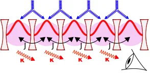
In this letter, we find the two-time correlations of a driven dissipative lattice, and see the emergence of a quasi-thermalized state. We calculate both on-site and inter-site correlations, giving access to the momentum resolved fluorescence spectrum of a driven coupled cav-ity array. In order to eliminate boundary and finite-size effects, we work always with the translationally in-variant infinite lattice. On-site calculations in a finite-size lattice have also been recently studied for the XXZ model [50]. While the methods we present are general, our work will focus on the transverse field anisotropic XY model (which has both the Ising and XY models as spe-cial cases), a driven dissipative realization of which was proposed by Bardyn and ˙Imamo˘glu [51], and the steady state properties studied [20, 52] using matrix product state approaches. As shown in [51] and reviewed in the supplementary material [53], this model can be realized by an array of coupled cavities in the photon blockade regime, with a two-photon pump that creates pairs of photons in adjacent sites (see Fig. 6).

J

κ

J J J

κ κ κ

FIG. 1. Coupled cavity array with hoppingJ, photon lossκ

and two-photon pumping (blue line). When strong nonlinear-ity (purple shading) in each cavnonlinear-ity leads to photon blockade, this yields the transverse field anisotropic XY model [51].

Following [20, 53], working in the rotating frame of the pump, the effective Hamiltonian has the form: H =−JP

j

gσz

j +

1+∆ 2 σ

x

jσxj+1+

1−∆ 2 σ

y

jσ

y

j+1

. The di-mensionless transverse field g depends on the pump-cavity detuning, and the anistropy parameter ∆, given by the ratio of pump strength and photon hopping J. For ∆ = 1 we recover the Ising model and for ∆ = 0 the isotropic XY model. In the following we will work in units of J. For the driven system, the Hamiltonian is ac-companied by photon loss at rateκinto empty radiation modes. We thus have the master equation:

∂tρ=L{ρ}=−i[H, ρ]

+κ 2

X

j

2σ_j−ρσ_j+−σ+_jσ_j−ρ−ρ σ_j+σ_j−. (1)

While a non-driven system would equilibrate with the bath, the time-dependent driving breaks detailed bal-ance and leads instead to a nonequilibrium steady state (NESS).

The fluctuation and response spectra discussed above require evaluating two-time correlation functions which,

for a Markovian system, can be found using the quantum regression theorem [26]:

D

O₂(j)(t)O(₁i)(0)E= TrhO(₂j)etLO(₁i)ρss

i

, (2)

wherei, j label two lattice sites and 1,2 two local opera-tors. In order to compute this for an infinite lattice, we employ matrix product state (MPS) methods. We first find the steady stateρss of the master equation (1). We

do this by using the infinite Time Evolving Block Dec-imation (iTEBD) algorithm [54, 55] to find the trans-lationally invariant infinite MPS such thatL {ρss} = 0.

Starting from the NESS, we then calculate two-time cor-relations using Eq. (43). Because applying local oper-ators ˆO1 to ρss breaks translational invariance, we can

no longer propagate using iTEBD. For a finite size lat-tice, TEBD could be used, but this restricts the extent of correlations in both space and time, as excitations are re-flected from the boundaries [56]. Fortunately, a method to find such correlations in an infinite lattice has been developed by Ba˜nuls et al. [57] for unitary evolution. This approach [57], which we extend to open systems, writes the time evolution between applying ˆO1 and ˆO2

as a tensor network, and contracting this network gives the desired correlator (see [53] for details).

Using this approach, we calculate the fluctuation spectrum SO,O†(ω) and the response function of the

system χ00_O,O†(ω) which are at the heart of the

fluctuation-dissipation theorem [26, 41], SO,O†(ω) =

F(ω)χ00_O,O†(ω),with the distribution functionF(ω)

dis-cussed below. Both SO,O†(ω) and χ00

O,O†(ω) are the

Fourier transforms of two-time correlations

˜

SO,O†(t) =

1 2

D

{Oˆ(t),Oˆ†(0)}E, (3) ˜

χO,O†(t) =iθ(t)

D

[ ˆO(t),Oˆ†(0)]E, (4) which we may evaluate using Eq. (43).

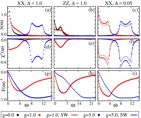
Figure 2 shows the on-site (i=j) fluctuation and re-sponse functions in frequency domain for ˆO1= ˆO2= ˆO∈

{σx_{, σ}z_{} and a range of values of transverse field g. We}

show both the Ising limit, (∆ = 1, left two columns) as well as at small ∆ (right column), where analytic results can be found using spin-wave theory as discussed fur-ther below. The panels (a–c) showS(ω) which measures the occupations while, panels (d–f) show response func-tionχ00(ω), which measures the density of states (DoS). We note that while at g = 0,1 we see S(ω) for σx is peaked atω= 0, its value always remains finite as there is no phase transition in this open one-dimensional sys-tem [20, 25]. As we will discuss later, the form of the density of states seen here can be understood from the momentum resolved correlation functions.

The bottom row of Fig. 2 shows the inverse distribution functionsF(ω)−1_=χ00

O,O†(ω)/SO,O†(ω) for ˆO=σx, σz

0.0 1.0

(a)

S(

ω

)

XX, ∆ = 1.0

0 0.2 0.4 0.6 0.8 1 1.2 1.4

(b) ZZ, _∆ = 1.0

0 0.2 0.4 0.6 0.8 1 1.2 1.4

(c) XX, _∆ = 0.05

-0.6 0.0

(d)

χ

"(

ω

)

-0.8 -0.7 -0.6 -0.5 -0.4 -0.3 -0.2 -0.1 0

(e)

-0.8 -0.7 -0.6 -0.5 -0.4 -0.3 -0.2 -0.1 0

(f)

-1.0 0.0

0 4 8 12 (g)

F(

ω

)

-1

ω

-1 -0.8 -0.6 -0.4 -0.2 0

0 7 14 21 (h)

ω

-1 -0.8 -0.6 -0.4 -0.2 0

0 4 8 12

(i)

ω

g=1.0 g=1.0, SW g=5.0 g=5.0, SW

g=0.0

FIG. 2. Spectrum of fluctuations S(ω), imaginary part of response function χ00(ω), and inverse distribution function

F(ω)−1. Left two columns: Ising limit ∆ = 1, Right column shows ∆ = 0.05 where spin-wave theory (solid lines) matches well. Energies given in units of J. Other parameters used:

κ= 0.5.

Fermionic or Bosonic (anti-)commutation relations; for Bosons it is: F(ω)≡2nB(ω) + 1 = coth((ω−µ)/2T).In

a driven dissipative system,F(ω) may take a more gen-eral form. However as identified in other contexts [7, 35– 41], quasi-thermalisation of low energy modes often oc-curs, leading to the identification of a low energy effective temperatureF(ω)∼2Teff/ω. Note that since all

calcula-tions are performed in the rotating frame, all frequencies are measured relative to the pump frequency — i.e. the pump frequency acts as an effective chemical potentialµ that sets the frequency at whichF(ω) diverges.

As seen in Fig. 2(g,h),F(ω)−1_{is linearω→0}

indicat-ing the emergence of a low energy effective temperature in this model. Because the power spectrum of physi-cal operators is positive, there is a minimum possible fluctuation contribution for a given dissipation, mean-ing |F(ω)|−1 _{≤1. At high frequencies the distribution}

function of a fully thermalised system asymptotically ap-proaches this value. In our non-equilibrium system we see that in some cases the inverse distribution|F(ω)|−1

approaches 1 over a range of frequencies, however in all cases it falls falls below one at higher frequencies, in-dicating higher fluctuations than for a thermal state. The results shown give some indication that, at least for Fig. 2(g), the F(ω) approaches a thermal form more closely at largerg.

The right column of Fig. 2 compares the MPS results (points) to analytic spin-wave theory [53, 58], which is valid if the density of excitations is small. We see a good agreement between spin-wave theory and MPS

numer--6 -4 -2 0

0 2 4

(a) T_eff, ∆ = 1.0

Teff

g

T_xx

T_zz

-6 -4 -2 0

0 3 6 9

(b) Teff, ∆ = 0.05

Teff

g

Txx

T_yy -g/2

FIG. 3. The effective temperatureTeffagainst transverse field

g. We find Teff by fitting F(ω) ' Acoth(bω) for low fre-quencies (ω ≤1.0), and plottingTeff ≡ A/2b. (a) MPS re-sults forσx,z _{fluctuations and the transverse-field Ising limit} (∆ = 1.0); (b) Spin wave results for σx,y _{fluctuations at} ∆ = 0.05. Energies given in units of J. Other parameters used:κ= 0.5.

ics at ∆ = 0.05 forσx _{correlations (we do not show the}

σz _{spectra for this ∆, as these vanish in the linearised}

spin-wave theory). Remarkably, the agreement forF(ω) is better than forS(ω), χ00(ω) individually. It is notable that despite being a linear (i.e. non-interacting) theory, the spin-wave result reproduces both the low energy ef-fective temperature and the emergent plateauF(ω)'1 at intermediate frequencies. The distribution function of spin-wave theory can be understood as a weighted aver-age ofk-dependent functionF(ω, k) = (2Teff,k+λkω2)/ω,

with weighting by thek-dependent density of states [53]. This form (which follows directly from the structure of the relevant linearised theory) leads directly to the exis-tence of a low energy effective temperature. The plateau at F(ω)' 1, seen only at larger g, results from the lo-cal spectra averaging over many momentum states [53], however the formF(ω, k) inevitably leads to F(ω)∝ω at high frequencies, corresponding to the breakdown of the plateau.

As well as the deviation from the thermalF(ω), a sec-ond distinction from an equilibrated system is that both the distribution and the low-energy effective temperature extracted differ depending on the system operator con-sidered. Figure 3(a) shows howTeffofσxandσz

correla-tors vary with transverse fieldg. Fig. 3(b) shows similar results for the spin-wave theory at small ∆ for σx _and

σy _{correlators (as noted above,σ}z _{correlators vanish in}

a linearised theory). We observe that for ∆→0,g→ ∞ theσx,y _{excitations thermalize to the same effective}

tem-perature, Teff ≈ −g/2. This can be understood asTeff,k

becomeskindependent in this limit, see [53].

-14 -7 0 7 14

ω

0 10 20 30

(a) S_xx(ω,k), g=5.0

-20 -10 0 10 20

0 0.2 0.4 0.6

(b) S_zz(ω_{,k), g=5.0}

-π _-π_{/2 0} π_/2 π

k

-4 0 4 8

ω

0 30 60 90 (c) S_xx(ω_{,k), g=1.0}

-π _-π_{/2 0} π_/2 π

k

-5 0 5 10

0 3 6 9

(d) S_zz(ω_{,k), g=1.0}

FIG. 4. S(ω, k) momentum-resolved fluctuation spectrum for excitations of: (a)σx atg= 5.0; (b)σz at g=5.0; (c)σx at

g= 1.0; (d)σz atg= 1.0. Energies given in units ofJ. Other parameters used: κ= 0.5.

note that fluctuation and dissipation spectra show differ-ent parity; χ00(−ω) = −χ00_{(ω), while S(−ω) = S(ω),}

and soF(−ω) =−F(ω). As such, the energy sign rever-sal underg7→ −gyields a sign change of the distribution function and effective temperature. We find g <0 gives positive temperatures, andg >0 negative temperatures. This is consistent with the spatial ordering seen [20]: for Teff <0 there is a high energy anti-ferromagnetic state.

A more intuitive understanding of this comes from the fact thatg is proportional to the pump-cavity detuning, so that g < 0 corresponds to a red-detuned pump and consequent cooling, whileg >0 corresponds to blue de-tuning. Blue-detuned pumping is typically associated to heating; here it does lead to energy accumulation, but this induces a negative temperature state, rather than high positive temperatures. At g= 0, the susceptibility χ00(ω) vanishes, soF(ω)−1_{= 0 and the effective}

temper-ature diverges.

So far we have evaluated correlation functions at equal positions; this corresponds to recording all light from one cavity, which implicitly integrates over momentum. More information on the structure of the correlations is avail-able if we consider the momentum-resolved spectrum. This requires evaluating correlations at non-equal sites i, j, and performing a double Fourier transform with re-spect to separation in timet and space|i−j|. The re-sulting fluctuation spectraS(ω, k) are displayed in Fig. 4 (The response function χ00(ω, k) shows similar features as S(ω, k)). We show the case for ˆO =σx_{, σ}z_{, and two}

values of g (we consider only g > 0, since the duality discussed above allows one to understand the effects of a sign change ofg). All the features visible in these spectra can be described straightforwardly using excitation

spec-tra derived from the Jordan-Wigner solution ofHTFI(see

e.g. [60] for details).

At large positive g, the NESS is known [20] to be a maximum energy state with spins pointing in the −ˆz direction, opposing the magnetic field. The spectrum of the σx _{operator corresponds to single spin flips, so}

follows the single particle dispersion ω(k) = (k) ≡ 2Jp1 +g2_{+ 2gcos(k) (where we considerde-excitations}

of themaximumenergy state). This expression is shown by the black line in Fig. 4(a). In contrast, theσz

oper-ator corresponds to two-particle excitations, which come in two varieties. The first one is a two-particle contin-uum withω=(k1) +(k2), k1+k2 =k. The envelope

of these states is given bymin(k)< ω(k)< max(k) with

max/min(k) = 4J

p

1 +g2_{±2gcos(k/2), shown by the}

dotted black lines in Fig. 4(b). The other kind of exci-tations involves scattering existing particles from mode qto q+k, i.e. ω(k) = ∆(q, k)≡ (q+k)−(q). The dominant contribution comes fromq= 0, since this cor-responds to the maximum energy mode, which is max-imally occupied for a negative temperature state. The black solid line shows ∆(0, k) which indeed matches the dominant feature observed. Given these momentum re-solved results, the momentum integrated spectral func-tions in Fig. 2(a,c) can be easily understood, with peaks arising from van Hove singularities at the band edges.

Near g = 1.0 the NESS instead shows antiferromag-netic correlations. The spectra here retain key features but are distorted. In the σx spectrum, Fig. 4(c) and Fig. 2(a,c), the peaks atk =±π become dominant. In theσz spectrum, Fig. 4(d) and Fig. 2(b,d), the scatter-ing band and two-particle continuum overlap. The black lines show the same expressions as discussed above. A ground state phase transition occurs for |g| < 1, hence the gap closing at g = 1.0. In contrast, the NESS at g = 1.0 already enters an antiferromagnetic state. As such, it is unsurprising these dispersions (which use nor-mal state Jordan Wigner forms) do not match the spec-trum as well as they did atg= 1.0. As one continues to decreaseg→0 the spectrum becomes further dominated by the modes nearω= 0, as seen in Fig. 2(a–d).

correla-tions may also be of interest, in revealing the coherence and statistics of any ordered state. Our results illustrate how calculating such correlations of the fluorescence can provide new insights into the state of many-body driven dissipative systems.

DK acknowledges support from the EPSRC CM-CDT (EP/L015110/1). JK acknowledges support from EP-SRC program TOPNES (EP/I031014/1). We are grate-ful to M. Hartmann and S. H. Simon for helpgrate-ful discus-sions, and to M. Hartmann for helpful comments on the manuscript.

[1] M. C. Cross and P. C. Hohenberg, Rev. Mod. Phys.65, 851 (1993).

[2] I. Bloch, J. Dalibard, and W. Zwerger, Rev. Mod. Phys. 80, 885 (2008).

[3] H. Ritsch, P. Domokos, F. Brennecke, and T. Esslinger, Rev. Mod. Phys. 85, 553 (2013).

[4] A. J. Daley, Adv. Phys.63, 77 (2014).

[5] T. Langen, R. Geiger, and J. Schmiedmayer, Annu. Rev. Condens. Matter Phys.6, 201 (2015).

[6] M. Mitrano, A. Cantaluppi, D. Nicoletti, S. Kaiser, A. Perucchi, S. Lupi, P. D. Pietro, D. Pontiroli, M. Ricc, S. R. Clark, D. Jaksch, and A. Cavalleri, Nature 530, 461 (2016).

[7] I. Carusotto and C. Ciuti, Rev. Mod. Phys. 85, 299 (2013).

[8] S. Schmidt and J. Koch, Ann. Phys. (Berlin)525, 395 (2013).

[9] C. Noh and D. G. Angelakis, Rep. Prog. Phys.80, 016401 (2016).

[10] M. J. Hartmann, Journal of Optics18, 104005 (2016). [11] A. Majumdar, A. Rundquist, M. Bajcsy, and

J. Vuˇckovi´c, Phys. Rev. B86, 045315 (2012).

[12] V. G. Sala, D. D. Solnyshkov, I. Carusotto, T. Jacqmin, A. Lemaˆıtre, H. Ter¸cas, A. Nalitov, M. Abbarchi, E. Ga-lopin, I. Sagnes, J. Bloch, G. Malpuech, and A. Amo, Phys. Rev. X5, 011034 (2015).

[13] K. Toyoda, Y. Matsuno, A. Noguchi, S. Haze, and S. Urabe, Phys. Rev. Lett.111, 160501 (2013).

[14] A. A. Houck, H. E. T¨ureci, and J. Koch, Nature Physics 8, 292 (2012).

[15] M. Fitzpatrick, N. M. Sundaresan, A. C. Y. Li, J. Koch, and A. A. Houck, Phys. Rev. X7, 011016 (2017). [16] I. Carusotto, D. Gerace, H. Tureci, S. De Liberato,

C. Ciuti, and A. ˙Imamo˘glu, Phys. Rev. Lett.103, 033601 (2009).

[17] M. J. Hartmann, Phys. Rev. Lett.104, 113601 (2010). [18] T. Grujic, S. Clark, D. Jaksch, and D. Angelakis, New

J. Phys.14, 103025 (2012).

[19] F. Nissen, S. Schmidt, M. Biondi, G. Blatter, H. E. T¨ureci, and J. Keeling, Phys. Rev. Lett. 108, 233603 (2012).

[20] C. Joshi, F. Nissen, and J. Keeling, Phys. Rev.A 88, 063835 (2013).

[21] J. Jin, D. Rossini, R. Fazio, M. Leib, and M. J. Hart-mann, Phys. Rev. Lett.110, 163605 (2013).

[22] J. Jin, D. Rossini, M. Leib, M. J. Hartmann, and R. Fazio, Phys. Rev.A 90, 023827 (2014).

[23] A. Biella, L. Mazza, I. Carusotto, D. Rossini, and R. Fazio, Phys. Rev.A91, 053815 (2015).

[24] M. Schir´o, C. Joshi, M. Bordyuh, R. Fazio, J. Keeling, and H. T¨ureci, Phys. Rev. Lett.116, 143603 (2016). [25] T. E. Lee, S. Gopalakrishnan, and M. D. Lukin, Phys.

Rev. Lett.110, 257204 (2013).

[26] H.-P. Breuer and F. Petruccione, The theory of open quantum systems (Oxford University Press, Oxford, 2002).

[27] A. N. Vamivakas, Y. Zhao, C.-Y. Lu, and M. Atat¨ure, Nature Physics5, 198 (2009).

[28] C. Lang, D. Bozyigit, C. Eichler, L. Steffen, J. M. Fink, A. A. Abdumalikov, M. Baur, S. Filipp, M. P. da Silva, A. Blais, and A. Wallraff, Phys. Rev. Lett.106, 243601 (2011).

[29] T. C. H. Liew and V. Savona, Phys. Rev. Lett. 104, 183601 (2010).

[30] M. Bamba, A. Imamo˘glu, I. Carusotto, and C. Ciuti, Phys. Rev. A83, 021802 (2011).

[31] S. R. K. Rodriguez, W. Casteels, F. Storme, N. Car-lon Zambon, I. Sagnes, L. Le Gratiet, E. Galopin, A. Lemaˆıtre, A. Amo, C. Ciuti, and J. Bloch, Phys. Rev. Lett.118, 247402 (2017).

[32] T. Fink, A. Schade, S. H¨ofling, C. Schneider, and A. ˙Imamo˘glu, Nature Physics14, 365 (2018).

[33] C.-K. Chan, T. E. Lee, and S. Gopalakrishnan, Phys. Rev.A91, 051601 (2015).

[34] F. Iemini, A. Russomanno, J. Keeling, M. Schir`o, M. Dal-monte, and R. Fazio, Phys. Rev. Lett. 121, 035301 (2018).

[35] S. Diehl, A. Micheli, A. Kantian, B. Kraus, H. B¨uchler, and P. Zoller, Nat. Phys.4, 878 (2008).

[36] S. Diehl, A. Tomadin, A. Micheli, R. Fazio, and P. Zoller, Phys. Rev. Lett.105, 015702 (2010).

[37] B. ¨Oztop, M. Bordyuh, ¨O. E. M¨ustecaplıo˘glu, and H. E. T¨ureci, New J. Phys.14, 085011 (2012).

[38] E. G. D. Torre, S. Diehl, M. D. Lukin, S. Sachdev, and P. Strack, Phys. Rev.A87, 023831 (2013).

[39] M. Buchhold, P. Strack, S. Sachdev, and S. Diehl, Phys. Rev.A87, 063622 (2013).

[40] L. Sieberer, S. Huber, E. Altman, and S. Diehl, Phys. Rev. Lett.110, 195301 (2013).

[41] L. M. Sieberer, M. Buchhold, and S. Diehl, Rep. Prog. Phys.79, 096001 (2016).

[42] J. Klaers, J. Schmitt, F. Vewinger, and M. Weitz, Nature 468, 545 (2010).

[43] P. Kirton and J. Keeling, Phys. Rev.A91, 033826 (2015). [44] T. D. Doan, H. T. Cao, D. B. Tran Thoai, and H. Haug,

Phys. Rev. B72, 085301 (2005).

[45] J. Kasprzak, D. D. Solnyshkov, R. Andr´e, L. S. Dang, and G. Malpuech, Phys. Rev. Lett.101, 146404 (2008). [46] Y. Sun, P. Wen, Y. Yoon, G. Liu, M. Steger, L. N.

Pfeif-fer, K. West, D. W. Snoke, and K. A. Nelson, Phys. Rev. Lett.118, 016602 (2017).

[47] A. Polkovnikov, K. Sengupta, A. Silva, and M. Vengalat-tore, Rev. Mod. Phys.83, 863 (2011).

[48] J. Eisert, M. Friesdorf, and C. Gogolin, Nat. Phys.11, 124 (2015).

[49] T. Langen, T. Gasenzer, and J. Schmiedmayer, J. Stat. Mech. Theor. Exp.2016, 064009 (2016).

dynamics,” (2018), preprint, 1809.10464.

[51] C.-E. Bardyn and A. ˙Imamo˘glu, Phys. Rev. Lett. 109, 253606 (2012).

[52] E. Mascarenhas, H. Flayac, and V. Savona, Phys. Rev.A 92, 022116 (2015).

[53] Supplementary Material containing derivation of the ef-fective model, details of the spin wave calculation, and a full description of the tensor network method for two-time correlations.

[54] U. Schollw¨ock, Ann. Phys.326, 96 (2011). [55] R. Or´us, Ann. Phys.349, 117 (2014).

[56] H. N. Phien, G. Vidal, and I. P. McCulloch, Phys. Rev.B 86, 245107 (2012).

[57] M. C. Ba˜nuls, M. B. Hastings, F. Verstraete, and J. I. Cirac, Phys. Rev. Lett.102, 240603 (2009).

[58] D. C. Mattis, The theory of magnetism made simple: an introduction to physical concepts and to some useful mathematical methods(World Scientific Publishing Com-pany, 2006).

[59] A. C. Y. Li and J. Koch, New Journal of Physics 19, 115010 (2017).

[60] S. Sachdev,Quantum phase transitions(Cambridge Uni-versity Press, Cambridge, 2007).

[61] M. O. Scully and M. S. Zubairy,Quantum Optics (Cam-bridge, 1997).

[62] G. Ford and R. O’Connell, Phys. Rev. Lett. 77, 798 (1996).

[63] A. Altland and B. D. Simons, Condensed matter field theory (Cambridge University Press, Cambridge, 2010). [64] E. Stoudenmire and S. R. White, New J. Phys. 12,

SUPPLEMENTARY MATERIAL FOR: FLUORESCENCE SPECTRUM AND THERMALIZATION IN A DRIVEN COUPLED CAVITY ARRAY

DRIVEN-DISSIPATIVE XY MODEL

This section provides the derivation of the effective transverse field anisotropic XY model which we study, starting from a model of a coupled cavity array, follow-ing Refs. [20, 51].

We consider a 1D lattice of optical or microwave cav-ities supporting photon modesbj with tunneling

ampli-tudeJ between adjacent cavities, and an on-site optical nonlinearityU which induces effective photon-photon in-teractions in each cavity. Such a coupled cavity array is thus described by the Bose-Hubbard Hamiltonian:

H =X

j

h

ωcb†jbj+U b

†

jb

†

jbjbj−J

b†_jb_j+1+ H.c.i.

In addition to these elements, we consider a two-photon drive Ω cos(2ωPt) near two-photon resonance ωP ≈ ωc.

We then work in the limit of strong optical nonlinearity with a perfect photon blockade, which restricts occupa-tions to at most one photon in each cavity. This strong nonlinearity then implies that the two-photon drive is only resonant with creation of photon pairs on adjacent cavities. The above considerations allow us to replace each cavity mode with a spin-1/2, equivalent to replac-ing the bosonic operators by Pauli matrices: bj → σ−j.

Our model Hamiltonian then becomes:

H0=

X

j

ωc

2 σ

z

j−J

X

j

σ_j+σ_j−₊₁+ H.c.

−ΩX

j

σ_j+σ_j+₊₁e−2iωpt_{+ H.c.. (5)}

If we then define the dimensionless parametersg= (ωp−

ωc)/2J, ∆ = Ω/J, we can transform H0 to a rotating

frame (at pump frequencyωp) to gauge away the explicit

time-dependence and write:

H=−JX

j

gσ_jz+1 + ∆

2 σ

x

jσ

x

j+1+

1−∆

2 σ

y

jσ

y

j+1

.

(6) The HamiltonianH of a coupled cavity array thus takes a form ofXY model wheregacts as the transverse mag-netic field, and ∆ is the anisotropy of spin-spin interac-tions. The limit ∆ = 0 corresponds to the isotropic XY model and ∆ = 1 to the Ising model.

SPIN-WAVE APPROXIMATION AT SMALL EXCITATION NUMBER

In this section we present further of the spin wave the-ory [58] used to describe the behavior at small excitation number. In particular, we can use this to understand ei-ther the limit of large|g|or small ∆, as both lead to small excitation number. Such an approach was used in Joshi et al.[20] for small ∆ to calculate static correlation tions; here we extend this to dynamical correlation func-tions and associated spectra.

At ∆ = 0 (i.e. zero pumping Ω/J = 0), or atg→ −∞, the NESS of our model corresponds to an empty state. For a small ∆, one can thus use spin-wave approxima-tion, which ignores the constraint on double occupancy of a lattice site, and so is only valid for a low density of excitations. In this small excitation number regime we can revert from spin-1/2 operators (hard-core bosons) to bosonic fields: σ_j− → bj, hence recovering aspects of a

weakly interacting model. (Note that for large positive g a similar argument can be made, making use of the duality underg→ −g discussed in the manuscript.)

Calculating correlation functions

Spin-wave approximation and equations of motion

We first follow the steps described in [20] to derive the Hamiltonian in terms of Bosonic system operators bk and b†−k. Working in the momentum basis, bk =

P

je

ikj_b

j/

√

N, the master equation, written as Eq. (1) in the main text becomes:

∂tρ=−i

X

k

[hk, ρ] +

κ 2

X

k

2ˆbkρb†k−b

†

kbkρ−ρ b†kbk

,

(7) where

hk=− b†_k b−k

g+ cos(k) ∆ cos(k) ∆ cos(k) g+ cos(k)

bk

b†_−k

, (8)

can be written in a matrix form:

∂tf(t) =M f(t) +v(t), (9)

with the vectors:

f(t) = _b

k(t)

b†_−k(t)

, v(t) =√2κ _bin

k(t)

b†₋in_k(t)

, (10)

and the matrix:

M =

−κ+ 2i(g+ cos(k)) 2i∆ cos(k) −2i∆ cos(k) −κ−2i(g+ cos(k))

.

(11) Here, coupling to Markovian bath introduces the input noise termbin

k(t). Since we consider a zero temperature

bath, there is only vacuum quantum noise, and the only nonzero correlator isDbin_k(t)b†_kin0 (t0)

E

=δk,k0δ(t−t0).

The solution of (9) is:

f(t) =eM tf(0) + Z t

0

dt0eM(t−t0)v(t0).

In the long-time limitt→ ∞we find the expressions for system operators:

bk(t) =

√ 2κ

Z t

0

dt0hG1(t−t0)bink(t

0_{) +G}

2(t−t0)b†₋in_k(t0)

i ,

b†_−k(t) =√2κ Z t

0

dt0hG∗₁(t−t0)b†₋in_k(t0) +G∗₂(t−t0)bin_k(t0)i. (12)

where the propagators G1,2(τ) are matrix elements of

eM t _{given by:}

G1(τ) =e−κτ

cos(ξkτ) +ik

sin(ξkτ)

ξk

, (13)

G2(τ) =iηke−κτ

sin(ξkτ)

ξk

, (14)

with dispersionsk = 2(g+ cos(k)),ηk= 2∆ cos(k), and

ξk=

p 2

k−η2k.

Correlations and effective temperatures for ˆσx

After deriving the system operators, we now proceed to calculate the frequency-resolved spectra for XX cor-relations. Sinceσx

j →bj+b†j in the spin-wave limit, we

can express the on-siteXX two-time correlator as:

˜

Cxx(τ) =hσx_(0)σx_(τ)i=

b†(0)b†(τ)

+hb(0)b(τ)i +b†(0)b(τ)+b(0)b†(τ), (15) where the correlations are given by a Fourier transform from momentum to real space:

b†(0)b(τ) =

Z π

−π

dk eiklDb†_k(0)bk(τ)

E _l=0

,

and similar expressions for other correlators. We then substitute in the solutions for operators (12), and evalu-ate the time integrals at unequal times,t+τandt. This gives a two-time correlator:

˜

Cxx(τ) =e

−κτ

2π Z π

−π

dk "

cos(ξkτ) +i(ηk−k)

sin(ξkτ)

ξk

+ηk(ηk−k) ξ2

k+κ2

cos(ξkτ) +κ

sin(ξkτ)

ξk

# . (16)

The quantities of interest are the fluctuation spec-trumS(ω) and susceptibilityχ00(ω) given by the Fourier transforms of ˜S(τ) = 1₂( ˜C(τ)∗ + ˜C(τ)) and ˜χ(τ) = iΘ(τ)( ˜C(τ)∗_{−C(τ)) respectively. Plugging in (16) and}˜ taking a Fourier transform with respect toτ, we obtain XX spectra:

Sxx(ω) =

κ π

Z π

−π

dk Pk+ω

2_{+ 2η}

k(ηk−k)

Qk(ω)

, (17)

χ00xx(ω) =

2κω π

Z π

−π

dk ηk−k

Q−_k1(ω), (18) where we have introduced auxiliary functionsPk=ξ2k+

κ2_{, andQ}

k(ω) = (Pk−ω2)2+ (2ωκ)2.

One can then substitute eik→z, and the integrals in (17), (18) become contour integrals around a unit circleC with|z|= 1. The values of (17), (18) are then determined by the residues of polesz=Z located insideC(i.e. with |Z|<1). Both (17) and (18) have the same set of eight poles given by:

Z=θs1,s2± q

θ2

s1,s2−1,

θs1,s2=

−g+s1

q

g2_∆2₋1−∆2

4 [κ2−ω2+s22iωκ]

1−∆2 ,

withs1=±1,s2=±1. Evaluating the contour integrals

gives fluctuation spectrum:

Sxx(ω) = 2κ

X

|Zn|<1

Znαn, (19)

where

αn =

(1−∆)Z_n2+ 2gZn+ (1−∆)

2

+ (ω2+κ2)Z_n2 (1−∆2₎2Q8

m=1,m6=n(Zn−Zm)

.

Similarly the susceptibility is given by:

χ00_xx(ω) =−4κω X

|Zn|<1

Z_n2βn, (20)

where

βn =

(1−∆)Z_n2+ 2gZn+ (1−∆)

(1−∆2₎2Q8

m=1,m6=n(Zn−Zm)

In both expressions, the sum runs over poles Zn inside

the unit circle C with |Zn| < 1. From (19) and (20)

it is straightforward to derive the distribution function Fxx(ω) of fluctuation-dissipation theorem:

Fxx(ω) =

Sxx(ω)

χ00

xx(ω)

=− 1 2ω

P

|Zn|<1Znαn

P

|Zn|<1Z

2

nβn

. (21)

It is evident that in the low frequency limit ω → 0, the distribution Fxx(ω) is dominated by the 1/ω

diver-gence. The effective thermalization of NESS thus already emerges in spin-wave theory, leading to an effective tem-peratureTeff:

Teff,xx=−

1 4

P

|Zn|<1Znαn

P

|Zn|<1Z

2

nβn

_ω=0

. (22)

Correlations and effective temperatures for ˆσy

Similarly to the previous subsection, we can calculate the fluctuation spectrum and susceptibility forY Y exci-tations in the spin-wave limit where σ_jy → −i(bj−b†j).

By following the same steps as for XX correlators, we obtain theY Y spectra:

Syy(ω) =

κ π

Z π

−π

dk Q−_k1(ω)

Pk+ω2+ 2ηk(ηk+k)

,

(23)

χ00_yy(ω) = 2κω π

Z π

−π

dk Q−_k1(ω)(ηk+k). (24)

The only differ from the expressions forXXspectra (17), (18) by (ηk −k) → (ηk +k). Note that as a result,

the contours integrals to evaluate have the same poles as forXX correlators, but with different residues and thus different weights.

Continuing along the same steps as forXXcorrelators, we find theY Y fluctuation spectrum:

Syy(ω) = 2κ

X

|Zn|<1

Znγn, (25)

where

γn=

(1 + ∆)Z2

n+ 2gZn+ (1 + ∆)

2

+ (ω2_+κ2_)Z2

n

(1−∆2₎2Q8

m=1,m6=n(Zn−Zm)

.

TheY Y susceptibility is given by:

χ00_yy(ω) =−4κω X

|Zn|<1

Z_n2δn, (26)

where

δn=

(1 + ∆)Z_n2+ 2gZn+ (1 + ∆)

(1−∆2₎2Q8

m=1,m6=n(Zn−Zm)

.

and the polesZnare the same as inXXspectra. One can

then straightforwardly derive the distribution function Fyy(ω):

Fyy(ω) =

Syy(ω)

χ00

yy(ω)

=− 1 2ω

P

|Zn|<1Znγn

P

|Zn|<1Z

2

nδn

. (27)

and the effective temperatureTeff:

Teff,yy=−

1 4

P

|Zn|<1Znγn

P

|Zn|<1Z

2

nδn

_ω=0

. (28)

Vanishing correlations forσz

Note that while the above approach allows calculation of theXXandY Y correlators, we cannot use this small excitation number approximation to find theZZ correla-tors. To see this, note that if we express theZZ two-time correlator usingσ_jz =b†_jbj−bjb†j, then in the spin-wave

limit:

˜

Czz(τ) =hσz_(0)σz_(τ)i=

=b†(0)b(0)b†(τ)b(τ)−

b(0)b†(0)b†(τ)b(τ) +

b(0)b†(0)b(τ)b†(τ) −

b†(0)b(0)b(τ)b†(τ) . (29)

Since the problem involves non-interacting bosons, the steady state is Gaussian and we can expand the four-field correlators using Wick’s theorem, which leads to

˜

Czz_{(τ) = 0. Thus, at this order of approximation allZZ}

spectra are trivially zero. This is to be expected, since σz correlations are quartic and the spin wave theory is linear.

Temperature of individual bosonic modes

Building on the spin-wave theory introduced above, we next discuss thermalization and the appearance of an effective temperature from this linear theory. To under-stand these effects, it is helpful to consider the contri-bution of individual bosonic modes. From (17), (18) we thus define the momentum-resolved fluctuation spectrum and susceptibility:

Sxx(ω, k) =

κ π Q

−1

k (ω)

Pk+ω2+ 2ηk(ηk−k)

. (30)

χ00_xx(ω, k) =2κω π Q

−1

k (ω)(ηk−k). (31)

Then the distribution function of an individual bosonic k-mode:

Fxx(ω, k) =

Sxx(ω, k)

χ00

xx(ω, k)

= ξ

2

k+ω

2_+κ2_{+ 2η}

k(ηk−k)

2ω(ηk−k)

.

Focusing on the frequency dependence of this expression, we see it can be written in the form:

Fxx(ω, k) =

2Teff,xx,k+λxx,kω2

ω , (33)

where λxx,k = [2(ηk−k)]−1, and the effective

temper-ature of an individual bosonic mode, defined from the ω→0 limit is:

Teff,xx,k =

κ2_{+ (η}

k−k)2

4(ηk−k)

, (34)

where we have used the definition ofξ2

k=2k−η2k.

From the above, we see that despite considering a lin-earized (i.e. non-interacting) theory, a low energy ef-fective temperature emerges for each individualkmode. However, the functional form ofFxx(ω, k) does not show

a plateau aroundFxx(ω, k)'1, as expected for an

equi-librium system, and as sometimes seen from the MPS numerics forFxx(ω). Instead|Fxx(ω, k)|−1shows a peak

at ω = ω∗_xx,k ≡ p

2Teff,xx,k/λxx,k =

p κ2_{+ (η}

k−k)2,

with a peak height

|Fxx(ωxx,k∗ , k)|

−1₌ 1

p

8Teff,xx,kλxx,k

= s

(ηk−k)2

κ2_{+ (η}

k−k)2

.

One may see that as required, this peak value is always less than one, and approaches one if damping is weak compared the energy difference|ηk−k|. While this

mo-mentum resolved distribution function does not show a plateau, as seen in Fig. 2, a plateau does arise for the site-local (i.e. momentum integrated) result. This site-site-local distribution function can be expressed as a weighted aver-age of distributionsF(ω, k) of individual bosonic modes:

F(ω) = Rπ

−πdk F(ω, k)χ

00_{(ω, k)}

Rπ

−πdk χ00(ω, k)

. (35)

Because the location of the peak for each mode k differs, this weighted average shows a plateau aris-ing from combinaris-ing all these peaks, stretcharis-ing over a range of frequencies, set by the range of peak frequencies, i.e. pκ2_{+ 4[g−(1−∆)]}2 _{< ω}∗

xx,k <

p

κ2_{+ 4[g−(1 + ∆)]}2_{. Note that as such the location}

of the plateau moves to higher frequencies as we increase g, as seen in Fig. (2) of the ma text. Note also that the plateau is always finite, and F(ω)∝ ω at large enough frequency.

As noted earlier, if we look atY Y correlations in place of XX, the only change is to replace ηk−k → ηk +

k in the above expressions, including in the density of

statesχ00(ω, k). Because of this change, one has both that

Teff,yy,k differs from Teff,xx,k, as well as the distribution

of occupied modes changing.

In the limit of large g, Eq. (34) becomes Teff,xx,k ≈

Teff,yy,k ≈ −g/2, independent of momentum k and the

operator being measured. Since this result is indepen-dent of momentum, the local effective temperature from Eq. (35) also approaches this value,

Teff≈ −g/2. (36)

In Fig.(3) of the main text we show the extracted tem-perature of the spin-wave theory for bothσxandσy

cor-relators: at large g, where quasi-thermalization holds, we see both temperatures approach this same value. In the opposite limit, of small g, one may note that ηk±k= 2(∆±1) cos(k)±g can now pass through zero

for some realk, leading to a divergence of bothTeff,kand

λk. This divergence is however integrable, giving a finite

form ofF(ω) and the correspondingTeff, except as seen

atg= 0 in Fig.(3).

Correlations for the Ising limit

As noted earlier, the small excitation density limit can be understood as resulting either from small ∆ or large g. As such, this approximation should remain valid even for the Ising limit, ∆ = 1, as long as g 1. However, at first appearance the above results are singular in the limit ∆ = 1. This is in fact not the case as one may readily check. For example, considering ˆO = ˆσx_{, we see}

that as ∆→1 the poles givenZ are still given byθs1,s2 but the values ofθs1,s2 become singular, specifically:

θs1,s2 = (

−(κ+s2iω)2/8g s1= +1

−g/(1−∆) s1=−1

.

Inserting this into the definition ofZ, we find that of the eight poles, four remain finite, while two tend to zero and two to infinity. Pairs of poles at zero and infinity in fact cancel, as long as the residue at the remaining poles is finite. This can be checked to be true, with the residues becomingαn = (ω2+κ2)/16g2 for the finite poles. The

behavior in the limit ∆→1 is shown in Fig. 5.

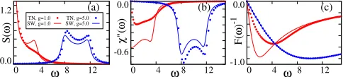
0.0 1.2

0 4 8 12

(a)

S(

ω

)

ω TN, g=1.0 SW, g=1.0 SW, g=5.0TN, g=5.0

-0.6 0.0

0 4 8 12

(b)

χ

"(

ω

)

ω -1.0

0.0

0 4 8 12

(c)

F(

ω

)

-1

ω

FIG. 5. Correlation functions for ∆ = 1, comparing MPS numerics (points) with spin wave calculations (lines). Panels (a-c) show the spectrum of fluctuationsS(ω), imaginary part of response functionχ00(ω), and the inverse distribution func-tionF(ω)−1 respectively. The results match well forg= 5.0, but poorly forg= 1.0.

hold. As with the small ∆ results in the main text, we see that the distribution function matches more accu-rately than the fluctuation and response functions sepa-rately. We may note that for ∆ = 1, there is never a true plateau in the distribution function. This can be under-stood from the fact that for ∆ = 1,k−ηk = 2g, so both

Teff,xx,k=−(κ2+ 4g2)/4gandλxx,k =−1/2gbecome

in-dependent ofk, meaning thatFxx(ω, k) is also

indepen-dent ofk, so the integrated versionF(ω) follows the form of Eq. (33), having a peak atω∗=pκ2_{+ 4g}2_{as is visible}

in Fig. 5. Note however that forY Y correlations the same statement would not be true, ask+ηk = 2g+ 4 cos(k)

isk-dependent.

Fluctuation-dissipation relation in linear theories

It is notable that, as discussed above, the linearized the spin-wave result predicts a low energy quasi-thermal dis-tribution with a non-zero effective temperature for XX and Y Y excitations. This is particularly notable in the light of papers, e.g. Ford and O’Connell [62] which sug-gest that the fluctuation dissipation theorem fails for a Markovian dissipation of a bath, and one would expect to find the effectiveF(ω) to be frequency independent, cor-responding approximately to zero temperature. This sec-tion discusses why the model we consider does not show such behavior. Specifically, as already noted, the struc-ture of distribution function is dependent on the mode considered. If in place of the XX and Y Y correlations we had directly considered correlations of the anihilation operators, ˜Cbb†(τ) = b(0)b†(τ), then we would have

found the distribution function Fbb†(ω) would be flat.

We first discuss this point, and why it is that XX and Y Y distribution functions are not flat. Since Ref. [62] also considers the analogue ofXX correlations, we then address further differences between the model discussed there and our results.

We first discuss the observation that the distribution function for correlators of annihilation and creation op-erators generally leads to a flat distribution. A quantum harmonic oscillator (with frequency Ω, and field oper-ators b, b†) interacting with a bath of radiation modes (with frequencyωk, field operatorsBk†,Bkfor each mode)

via coupling strength is described by the Hamiltonian

H = Ωb†b+X

k

ωkBk†Bk+

X

k

h

gkbBk†+ H.c.

i

. (37)

Heregk is the system-bath coupling strength. Using the

standard input-output formalism [61] in the Markovian limit we derive Heisenberg-Langevin equation of motion

∂tb(t) =−iΩb(t)−κb(t) +

√

2κbin(t), (38)

where the input noise operator bin_{(t) is introduced by}

coupling to Markovian bath. For a zero-temperature

bath there is only vacuum noise and the only non-zero correlator is bin(t)b†in(t0) = δ(t−t0). Next, one can obtain the steady-state solution (att→ ∞):

b(t) =√2κ Z t

−∞

dt0e−iΩ(t−t0)−κ(t−t0)bin(t). (39)

The only non-vanishing two-time correlator then is

hb(0)b†(τ)i=e−κ|τ|+iΩτ. (40) Taking a Fourier transform of the symmetrized cor-relator ˜S_bb†(τ) = 1

2

{b(0), b†_(τ)}

= e−κ|τ|+iΩτ _and

response function ˜χbb†(τ) = iθ(τ)b(0), b†(τ) =

iθ(τ)e−κ|τ|+iΩτ _{gives the fluctuation spectrum and}

sus-ceptibility:

S_bb†(ω) =χ00_bb†(ω) =

2κ

(ω−Ω)2_+κ2. (41)

Subsequently, one obtains a flat distribution spectrum for b,b†modes, in contrast to the quasi-thermal distribution of theXX andY Y modes:

Fbb†(ω) =

Sbb†(ω)

χ00

bb†(ω)

= 1. (42)

Our spin-wave equations differs from the above deriva-tion in that the spin-wave theory has anomalous terms proportional to ∆. However, the derivation above can be extended just as well to a linear theory with anoma-lous terms since its Hamiltonian can be diagonalized eas-ily using the Bogoliubov transformation [63]. The cru-cial difference that occurs in the spin wave theory dis-cussed above is our calculation ofXX and Y Y correla-tions, which mean fluctuation and dissipation terms in-volve sums and differences of correlatorshb(0)b†_(τ)iand

hb†_{(0)b(τ)i. Once these are both considered, the single}

mode functions results in Eq. (30–32) follow, giving a frequency dependent result.

As noted earlier, the above result is notable in con-nection to the argument by Ford and O’Connell [62] that quantum regression can never give a thermal spec-trum. The problem considered there is similar to ours in that there are anomalous terms (since no rotating-wave approximation is made in the system bath cou-pling), and the correlations considered are theXX cor-relations. However, there is a crucial difference in that Ref. [62] considers Ohmic rather than Markovian dissi-pation. This difference leads to the different conclusions of the previous section.

TENSOR NETWORK APPROACH FOR TWO-TIME CORRELATIONS

T(O

)

T

Λ(2)Γ(1)_Λ(1)Γ(2)_Λ(2)

...

...

O

O

...

...

δt

R

j

T(O1)

L

i

δ

t

x

t

δ

t

δt/2

FIG. 6. Tensor network used to evaluate two-time correla-tions, using boundary eigenvectors (orange) for calculating two-time correlations under non-unitary Liouvillian propaga-tor.

systems in the thermodynamic limit. We use quantum re-gression to calculate two-time correlations Eq. (43), start-ing from the NESS density matrix ρSS, represented by

a translationally invariant infinite MPS that was previ-ously computed using infinite TEBD algorithm [54, 55].

D

O(₂j)(t)O(₁i)(0)E= TrhO₂(j)etLO₁(i)ρss

i

. (43)

For a finite size lattice, one could still directly use TEBD algorithm to perform the time evolution in (43). How-ever, such direct propagation is incompatible with infinite TEBD: application of a local operatorO1 toρSS breaks

translational invariance. A naive solution would be to use a finite size extrapolation, which is prone to bound-ary and finite-size effects. In particular, the finite lattice size would restrict the extent of correlations in both space and time, as excitations will be reflected back from the boundaries, and the simulation will be no longer valid at later times [56]. Such simulation would also inccur an additional computational cost that scales linearly with the system size which will be inefficient for large lattices needed to approximate the thermodynamic limit, in com-parison to only two sites required in the infinite TEBD. Nonetheless, such a method has been recently used to calculate aging dynamics in the XXZ model [50].

Fortunately, it is possible to avoid these issues that arise due to finite size altogether. A method to compute two-time correlations in an infinite system directly (i.e. without resorting to a finite size extrapolation) has been proposed by Ba˜nuls et al [57] for unitary evolution in isolated systems. In our work, we extend this approach

to open quantum systems whose dynamics is governed by the quantum master equation for density matrices. We provide a brief description of the algorithm below.

The idea is to construct a network representing the en-tire time evolution, instead of evolving the MPS in time step by step. We start from an infinite MPS represent-ing vectorized NESS density matrix|ρssi and apply the

first operatorO₁(i)(0) at the initial timet= 0. Then, for every time evolution step we insert a propagator MPO. After repeating this for the required number of time steps we apply the second operatorO₂(j)(t) at the final timet. Taking the trace at the final time removes the dangling physical dimension at each site of the last MPO propaga-tor. This procedure produces a 2D tensor network that is infinite along the spatial axis but finite along the time axis, giving an unnormalized two-time two-point correla-tor:

D

O(₂j)(t)O₁(i)(0)E ∝ TN→∞TO1 T

|i−j|−1_T

O2 T

N→∞_,

(44) where T = is a transfer matrix of the evolved density matrix, andTO1,2 are transfer matrices containing an ap-plication of operatorsO1,2 at the initial and final times

at lattice sites i, j, as shown in Fig. 1(b) of the main text.

Since the network is translationally invariant,T is the same on every site (except at the sites where the op-erators are applied) and we may effectively replace the semi-infinite lattices, to the left and right of the sites where ˆO1 and ˆO2 act, by the left and right

eigenvec-tors ofT corresponding to its largest eigenvalueλ since limN→∞TN = λN|RihL|. In practice, we compute an

MPS approximation to the eigenvectors |Ri, hL| by us-ing the MPS-MPO power method. We multiply an ini-tial arbitrary MPS (oriented along the time axis) byT (represented as an MPO along the time axis) a suffi-cient number of times until it converges to|Ri, hL| for the right- and left-multiplication respectively. We trun-cate the MPS bonds after each multiplication using the method described in [64], performing truncation along the time axis. Once we have calculated |Ri and hL|, the resulting network is finite along both space and time axes. It can then be easily contracted using MPO-MPS and MPS-MPS multiplications [54, 64] to give any two-time two-point correlator:

D

O(₂j)(t)O(₁i)(0)E=

L|TO1T

|i−j|−1_T

O2|R

λ|i−j|+1 , (45)

normalized by trace Tr(ρ) =

L|T|i−j|+1_|R