doi:10.4236/sgre.2010.11006 Published Online May 2010 (http://www.SciRP.org/journal/sgre)
A Qualitative Perstective on Idempotency Defect of
Two Level System Interacting with Laser and
Quantized Field
Sayed Abdel-Khalek1,2, Mohammed Mohammed Ali Ahmed1,4, Waleed Nabeel Razek3, Abdel ShafyObada4 1Mathematics Department, Faculty of Science, Taif University, Taif, Saudi Arabia; 2Department of Mathematics, Faculty of Science, Sohag University, Sohag, Egypt; 3Mathematics Department, Physics Division, National Research Centre, Cairo, Egypt; 4Mathematics Department, Faculty of Science, Al-Azher University, Nassr City, Cairo, Egypt.
Email: [email protected]
Received March 22nd, 2010; revised May 13th, 2010; accepted May 13th, 2010.
ABSTRACT
Entanglement due to the interaction of a two level atom with a laser and quantized field is investigated. The role of the nonlinearity due to these interactions is discussed. It is found that the nonlinearity changes strongly the behavior of the entanglement also the detuning parameters have important role in the structure of the measure of entanglement. Keywords:Entanglement, Idempotency Defect, Two-Level System, Quantized
1. Introduction
Quantum information processing provides different way for manipulating information other than the classical one. This is related to entanglement, which plays an essential role in the quantum information such as quantum com-puting [1], teleportation [2], cryptography [3], dense cod-ing [4] and entanglement swappcod-ing [5]. Thus intensive efforts have been done to understand theoretically and experimentally the entanglement in quantum systems. For instance, the entanglement between two qubits in an arbitrary pure state has been quantified by the concur-rence [6] and Peres-Horodecki measure [7]. However, that of the mixed states is quantified by the average con-currence over all possible pure state ensemble decompo-sition. Additionally, the entropic relations are used in investigating the entanglement in quantum system. In this regard von Neumann entropy (NE) [8], linear en-tropy (LE) and the Shannon information enen-tropy (SE) [9] have been frequently used in treating entanglement in the quantum systems. The NE [10] and the LE [11] have been applied to the JCM. It is worth mentioning that the SE involves only the diagonal elements of the density matrix and in some cases it can give information similar to that obtained from the NE and LE.
The paper is prepared in the following order: In Section 2 we define the system Hamiltonian. In Section 3, we derive the time evolution operator and density matrix. In
Section 4 we investigate the atomic inversion and idem-potency defect (ID). In Section 5 we summarize the main results.
2. The System Hamiltonian
described by the Hamiltonian (1):
,
A F AF AL
H H H H H (1) where HA 0Sz is the atom Hamiltonian, HF
†
ˆ ˆ
Ca a
is the field Hamiltonian, †
2( ˆ ˆ )
AF
H S a a S is the atom-field Hamiltonian, and
( ) ( )
( )
2
L L L L
i t i t
AL r
H S e e S
is the atom-laser Hamiltonian.
The atomic transition frequency is denoted by o, the
frequencies of the cavity and laser fields are denoted by c
and L receptivity, and the laser field is assigned by the
phase L, the operator a aˆ ˆ
† is the annihilation(crea-tion) operator of the cavity field and obey the commuta-tion relacommuta-tion [ , ] 1a aˆ ˆ† , and r are the coupling constants
associated with the cavity field and the classically de-scribed laser field respectively which are assumed real. The
S
operators are the coherence operators for the atom, satisfying the following angular momentum commutation relations [ ,S Sij lm]SimjlSlj mi where i j l m, , , 1, 2,...3. Time Evolution Operator and Density
Matrix
To obtain the time evolution operator, we must eliminate the explicit time dependence of the previous Hamiltonian 1), we use the following unitary operator [13]
†
ˆ ˆ ( )( )
( ) i Lt L Sz a a,
T t e (2)
we redefine the Hamiltonian as :
†
† †
1
( ) ( ) ( ) ( )dT t .
H T t HT t iT t
dt
(3)
Then the Hamiltonian 1) will be in the following form:
† †
1 cˆ ˆ L z 2( ˆ ˆ ) 2( ), r
H a a S S a a S SS (4)
where c c l and l 0 l, if we consider the resonant pumping case 0l and rearrange the Hamiltonian terms, the Hamiltonian (4) becomes.
/ /
1
/ /
ˆ ˆ ˆ ˆ
2 ˆ ˆ 2
z C z
H rS a a a a S
a a S S
(5)
The new atomic operators set
/ / /
(Sz S Sx, SziS Sy, SziSy)
which obey the angular momentum commutation relations among themselves. The eigenvector of /
z x
S S is the dressed states of the atom in the laser field alone and the operators S/
and S/ are the corresponding raising and
lowering operators.
To associate the third and the fourth terms of H1 we
use the following unitary transformation:
† 1 ,
H P H P (6) where P is an atomic state dependent displacement op-erator of the cavity field state which is defined as :
† / 2c(a a Sˆ ˆ ) z
P e (7) Then the Hamiltonian 4) takes the following form:
2/ ˆ ˆ ˆ ˆ / / ,
2 16
z C
C
H rS a a a a S v S v
(8)
where
† 1 2
2 (ˆ ˆ) 2 2( ) †
0 0
( 1) ˆ ˆ . 2 ! !
c c
n m n
a a m n
n m c
v e e a a
n m
(9)We can drop 2
16 c
which has no effect in the dynam-ics of the system.
This Hamiltonian describes a two level system with energy levels separated by r coupled to a single quan-tized mode of radiation frequency c and there is an infinite sequence of probe resonance zones in the neigh-borhood of the Rabi sub harmonic resonances at
, 1, 2,....
c m
m
If we consider of the RWA, the slowly varying terms are identified and retained, in the m th resonance zone
/
S has the zero order time dependence ei t that is
ap-proximately canceled by the zero order time dependence
c m i
e of all field operators of the form a aˆ ˆ†m n m , for any n. The Hamiltonian for the mth resonance zone is:
†
† / / /
ˆ ˆ ( )
4
eff c z m m
H a a rS S f S f (10)
In this case, we recognize as the mth-order multiphoton Jaynes Cumming Hamiltonian where we consider
ˆ ( ) m m
f f n a ,
2 2 2 2 0( 1) ˆ ˆ ( )
2 !
c
c
f n e a a
destroys m photons of frequency c where Heff can be
further simplified by means of another rotating wave approximation (RWA),( as discussed in detail in [12-14]).
The time evolution operator is given by:
† †
† †
11 12 ˆ ˆ
ˆ ˆ ( ),
( )
21 22
( ) ( ) eff ( )
L
iH
i a a i a a
U t T t Pe P T t
U U e e U U
(11)
Lt L
( ) 11 1 ( ), 2 L i
U e A B D E
( ) 12 ( ) 21 ( ) 22 1 ( ), 2
1 ( ),
2
1 ( ),
2 L L L i i i
U e A B D E
U e A B D E
U e A B D E
(12) and , ) ( , ) ( ) ( , ) ( ) ( , ) ( 2 2 2 2 1 2 1 2 G t F e iG E G t E n f e iG D G t E m f e iG B G t F Ge A t m n i t m n i t m n i t m n i C C C C
(13)
where
sin( ) sin( ) cos( ) j , j , 1, 2
j j j
j j
t t
F t i E j
.
Also,
2 2
1 1
2
2 1 1
1
( ) 16 ( ( )) , 4 ( )! ( ) ( ), ( ) ( ) , ! m n
n v n
n k
n n m v n L
n
where, 2 1
1
( ) ( ), ( ) 2 c
v n v n m m , G v 2 and
2
( )
m n
L is the Laguerre function. At t0 the wave function of the system can be written as:
0 cos sin2 e 2 g
(14)
where is the superposition state parameter
2
exp( ) , 2 ! n n n n
(15)
with the mean photon number n2, then the wave function at any time t0 is given by
ˆ ˆ
( )( )
12 22
( ) 0
, ,
L L i a a
t U t
e U e U g
(16)
In the pure state case it is well known that the density matrix of the atom-field interaction can be written as:
ρ t t t (17) In order to analyze what happens to the two level
sys-tems interacting with laser and quantized field, we trace out field variables from the state (t)ρ and get the re-duced atomic density matrix of the system given by
,A F AF AF
ee eg
L
ge gg
t tr t t
L L t e e t e g
t g e t g g
(18) where
( ) ( ) 12 12 ( ) ( ) 12 22 ( ) ( ) 22 12 ( ) ( ) 22 11 , , , . L L L L L L L Li n i n
ee
i n i n
eg
i n i n
ge
i n i n
gg
t n e U U e n
t n e U U e n
t n e U U e n
t n e U U e n
(19)
4. Atomic Inversion and Idempotency Defect
Atomic inversion can be considered as the simplest im-portant quantity. It is defined as the difference between the probability of finding the atom in the exited state and in the ground state, the time dependent atomic inversion in the m resonance th
c
(
m )
is given by:
ee gg
W(t) t t (20) Finally the idempotency defect as a measure of entan-glement is written as:
(J)
t f
2 A
2 ee gg eg
Tr { (t)(1 (t)} 1 Tr ( (t))
2 2 (21)
In many cases of quantum information processing, one requires a state with high purity and large amount of en-tanglement. Therefore, it is necessary to consider the purity of the state and its relation with entanglement.
Here we use the idempotency defect, defined by linear entropy, as a measure of the degree of purity for a state
( )t
, in analogy to what is done for the calculation of the entanglement in terms of von Neumann entropy [15] which has similar behavior in the same cases.
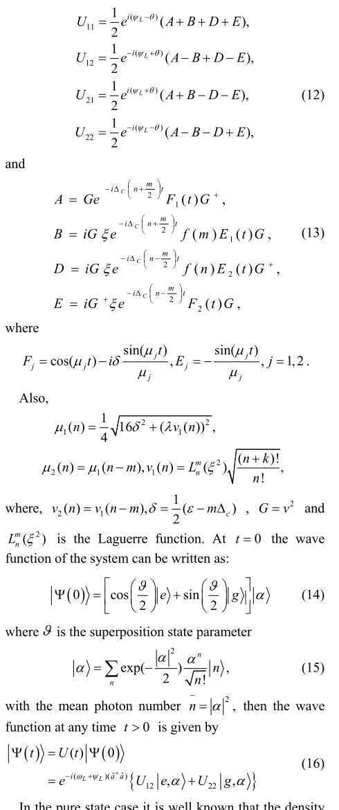
[In all our figures we have plotted the atomic inversion
W(t) and the entanglement ID (J)t as a function of the
[image:3.595.53.298.80.665.2]scaled time t for the case of two-photon processes]. In
0 20 40 60 80 100
−1 −0.5 0 0.5 1
W(t)
0 20 40 60 80 100
0 0.005 0.01 0.015 0.02 0.025 0.03 0.035
ζ
(t)
0 20 40 60 80 100
−1 −0.5 0 0.5 1
W(t)
0 20 40 60 80 100
0 0.1 0.2 0.3 0.4 0.5 0.6 0.7
ζ
(t)
The Laguerre function term is ignored
[image:4.595.123.470.101.370.2]The Laguerre function term is considered
Figure 1. The evolution of the (a) atomic inversion and idempotency defect against the scaled time rt for the parameters
α= 5 , ξ= 0.5, k = 2 the laser detuning parameter ΔC= 1 , 0 and = 0
0 100 200 300 400 500 600 700 800
−1 −0.5 0 0.5 1
W(t)
0 100 200 300 400 500 600 700 800
0 0.02 0.04 0.06 0.08 0.1 0.12 0.14
ζ
(t)
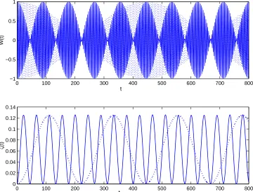
Figure 2. The evolution of the (a) atomic inversion and (b) idempotency defect against the scaled time rt for the parameters
α= 0 , ξ= 0.02 (dotted line), ξ= 0.1 (solid line), k = 2 the laser detuning parameter ΔC= 1 , 0 and = 0
t t
t t
t
[image:4.595.118.478.415.689.2]0 0.5 1 1.5 2 2.5 3 x 10⁴ −1
−0.5 0 0.5 1
W(t)
0 0.5 1 1.5 2 2.5 3
x 104 0
0.2 0.4 0.6 0.8 1
ζ
(t)
t
ζ=0.05
[image:5.595.135.463.87.349.2]ζ=0.01
Figure 3. The evolution of the (a) atomic inversion and (b) idempotency defect against the scaled time for the parameters = 10
, = 0.05 (dotted line), = 0.01 (solid line), k = 2 the laser detuning parameter ΔC= (2n - 0.5)π/ t, θ= 0 and δ= 0
0 500 1000 1500 2000 2500 3000 3500 4000
−1 −0.5 0 0.5 1
W(t)
0 500 1000 1500 2000 2500 3000 3500 4000
0 0.1 0.2 0.3 0.4 0.5 0.6 0.7
ζ
(t)
t
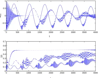
Figure 4. The evolution of the (a) atomic inversion and (b) idempotency defect against the scaled time rt for the parameters = 10
, k = 2 the laser detuning parameter ΔC= 1, 0 and with different values of the detuning = 0 (solid line),
= 0.01
(dashed line), = 0.1 (dotted line)
t
[image:5.595.136.461.411.670.2]0 2000 4000 6000 8000 10000 12000 −1
−0.5 0 0.5 1
W(t)
0 2000 4000 6000 8000 10000 12000
0 0.1 0.2 0.3 0.4 0.5 0.6 0.7
ζ
(t)
ζ=0.1
[image:6.595.90.508.90.407.2]ζ=0.01
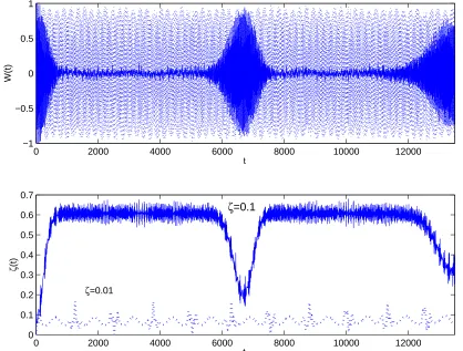
Figure 5. The evolution of the (a) Atomic inversion and (b) Idempotency defect against the scaled time, rt for the parameters
α= 10 , = 0.01 (dotted line), = 0.1 (solid line), k = 2 the laser detuning parameter ΔC= 1 , 0 and = 0.1
features of both the atomic inversion and ID are washed out, where as the time goes on the atomic inversion shows small amplitude of the oscillations and steady state of the ID (see
Figure 1). As the time increases further the maximum entangled state can be obtained, where W t( ) 0
( ) ( )
ee gg
ρ t ρ t at this moment the entanglement reaches its maximum value. An interesting case is seemed in Fig-ure 2, where we have considered small values of the pa-rameter . In this case the collapse-revival phenomenon is shown. Also, the periodic oscillation occurs each 60 for atomic inversion and the zero ID at 15 for = 0.1.
Now we shed the some light on the affect of the dif-ferent parameters on the both of the atomic inversion and the corresponding ID. For example the effect of the de-tuning C is considered in Figure 3. In this case we see that the amplitude of the value of the detuning increased as the value of the detuning increased. The ID decreases and reaches steady state as C increases further.
On the other hand, the detuning of the quantized field , plays the opposite role, where the ID shows steady state at maximum instead of lowing its value due to the detuning of the laser field.
As increases further (say = 0.5) we obtain a long
lived entanglement, as to show the fixed value of the ID ( = 0.5). In Figure 5, we see that the collapse-revival phenomenon is clearly seen. Also, a perfect correspon-dence between the atomic inversion revival and the local maxima corresponds to the collapse periods. Also, we see that the collapse-revival phenomenon is clearly seen. Also, a perfect correspondence between the atomic inversion revival and the local maxima corresponds to the collapse periods. we have plotted the atomic inversion and the corresponding field Idempotency for a state of mean photon number of the coherent field as n 10 , fixed the detuning parameter c 1 and the parameter = 0 and
changed the parameter with values (0.01 and 0.1), when = 0.01, oscillated with period equal t 2000 and W(t) oscillated with same interval and (J)
t
has a
long-lived entanglement in each interval. When = 0.01, then (J)
t
has a weak oscillation and W(t) oscillated with a very small interval between maximum and minimum values.
5. Conclusions
In the present paper we show that the on idempotency defect can be used to quantify entanglement of a two level
t
system interacting with laser and quantized field. We obtain the long living entanglement due to the idempo-tency defects of the field. Our results show that the non-linearity changes strongly the behavior of the entangle-ment also the detuning parameters have important role in the structure of the measure of entanglement. Also, all the interaction parameters play an important role on the be-havior of idempotency defect.
REFERENCES
[1] G. Benenti, G. Casati and G. Strini “Principles of Quan- tum Computation and Information, Vol. 1,” World Scien- tific, 2004.
[2] C. Bennet, G. Brassard, C. Crepeau, R. Jozsa, A. Peres and W. K. Wootersm, “Teleporting an Unknown Quan- tum State via Dual Classical and Einstein-Podolsky- Rosen Channels,” Physical Review Letter, Vol. 70, No. 13, 1993, pp.1895-1899 .
[3] A. Ekert, “Quantum Cryptography Based on Bell’s Theorem,” Physical Review Letter, Vol. 67, No. 6, 1991, pp. 661-663.
[4] L. Ye and G.-C. Guo, “Scheme for Implementing Quan- tum Dense Coding in Cavity QED,” Physical Review Letter A, Vol. 346, No. 5-6, 2005, pp. 330-336.
[5] O. Glöckl, S. Lorenz, C. Marquardt, J. Heersink, M. Brownnutt, C. Silberhorn, Q. Pan, N. V. Loock, N. Korolkova and G. Leuchs, “Experiment towards Continu- ous-Variable Entanglement Swapping: Highly Correlated Four-Partite Quantum State,” Physical Review Letter A, Vol. 68, No. 1, 2003, pp. 012319-012327.
[6] W. K. Wootters, “Entanglement of Formation of an Arbitrary State of Two Qubits,” Physical Review Letter, Vol. 80, No. 10, 1998, pp. 2245-2248.
[7] A. Peres, “Separability Criterion for Density Matrices,” Physical Review Letter, Vol. 77, No. 8, 1996, pp. 1413- 14150.
[8] J. von Neumann, “Mathematical Foundations of Quantum Mechanics,” Princeton University Press, Princeton, 1955. [9] C. E. Shannon and W. Weaver, “The Mathematical
Theory of Communication,” Urbana University Press, Chicago, 1949.
[10] S. J. D. Phoenix and P. L. Knight, “Fluctuations and Entropy in Models of Quantum Optical Resonance,” Annals of Physics, Vol. 186, No. 2, pp. 381-407, 1988. [11] F. A. A. El-Orany and A.-S. Obada, “On the Evolution of
Superposition of Squeezed Displaced Number States with the Multiphoton Jaynes–Cummings Model,” Jounal of Optics B: Quantum Semiclass Optics, Vol. 5, No. 1, 2003, pp. 60-72.
[12] M. Lewenstein and T. W. Mossberg, “Spectral and Statistical Properties of Strongly Driven Atoms Coupled to Frequency-Dependent Photon Reservoirs,” Physical Review Letter A, Vol. 37, No. 2048, 1988, pp. 2048-2062. [13] C. K. Law and J. H. Eberly, “Response of a Two-Level
Atom to a Classical Field and a Quantized Cavity Field of Different Frequencies,” Physical Review Letter A, Vol. 43, No. 11, 1991, pp. 6337-6344..
[14] J. H. Eberly and V. D. Popov, “Phase-Dependent Pump-Probe Line-Shape Formulas,” Physical Review Letter A, Vol. 37, No. 6, 1988, pp. 2012-2016.
[15] G. M. A. Al-Kader and M. M. A. Ahmad, “On the Interaction of Two-Level Atoms with Squeezed Coherent State,” Chinese Jounal of Physical, Vol. 39, No. 1, 2001, pp. 50-63.