Continuum limits of pattern formation in hexagonal cell monolayers

Continuum limits of pattern formation in

hexagonal-cell monolayers

R.D. O’Dea and J.R. King

Centre for Mathematical Medicine and Biology,

School of Mathematical Sciences,

University of Nottingham, University Park,

Nottingham, NG7 2RD, UK

June 10, 2015

Abstract

Intercellular signalling is key in determining cell fate. In closely packed tissues such as epithelia, juxtacrine signalling is thought to be a mechanism for the gener-ation of fine-grained spatial patterns in cell differentigener-ation commonly observed in early development.

Theoretical studies of such signalling processes have shown that negative feed-back between receptor activation and ligand production is a robust mechanism for fine-grained pattern generation and that cell shape is an important factor in the re-sulting pattern type. It has previously been assumed that such patterns can be anal-ysed only with discrete models since significant variation occurs over a lengthscale concomitant with an individual cell; however, considering a generic juxtacrine sig-nalling model in square cells, in O’Dea & King (Multiscale analysis of pattern

formation via intercellular signalling, Accepted in Math. Biosci.), a systematic

method for the derivation of a continuum model capturing such phenomena due to variations in a model parameter associated with signalling feedback strength was presented. Here, we extend this work to derive continuum models of the more complex fine-grained patterning in hexagonal cells, constructing individual mod-els for the generation of patterns from the homogeneous state and for the transi-tion between patterning modes. In additransi-tion, by considering patterning behaviour under the influence of simultaneous variation of feedback parameters, we con-struct a more general continuum representation, capturing the emergence of the patterning bifurcation structure. Comparison with the steady-state and dynamic behaviour of the underlying discrete system is made; in particular, we consider pattern-generating travelling waves and the competition between various stable patterning modes, through which we highlight an important deficiency in the abil-ity of continuum representations to accommodate certain dynamics associated with discrete systems.

1

Introduction

and mechanics with self-evident application to, for instance, in vitro tissue engineering or the understanding of tumour growth and invasion.

It is well known that cell-signalling mechanisms regulate differentiation, cell-fate determination and, ultimately, tissue and organ development. Such regulation is me-diated by the production, transport and binding of intercellular signalling molecules, which may be free to diffuse throughout the tissue or may be anchored in the cell membrane. In the latter case, cell-signalling molecules may bind only to directly adja-cent cells; such a juxtacrine signalling mechanism is therefore of particular interest in closely packed structures such as epithelia.

Lateral inhibition is a juxtacrine pattern-forming mechanism employed by devel-oping tissues to create fine-grained patterns of cell differentiation, in which adjacent or nearby cells diverge to achieve differing cell fates. This mechanism is controlled by a negative feedback loop: receipt of inhibition reduces the ability of a cell to inhibit others, leading to the amplification of differences between cells. This mechanism is evolutionarily conserved and is observed in insects, nematode worms and vertebrates, in all of which the transmembrane proteins Notch and Delta (or their homologues) have been identified as mediators of the interaction (see Collier et al (1996) and biological references therein). Well studied examples of such fine-grained patterns include com-pound eye and nervous tissue development in insects, such as the fruit fly, Drosophila (Haddon, 1998; Appel et al, 2001; Carthew, 2007). Within the context of regener-ative medicine, Delta-Notch signalling has been shown to regulate cell fate in stem cell clusters (Lowell et al, 2000). While other ligand-receptor interaction-mediated cell signalling mechanisms have been characterised (e.g. the binding of cyclic AMP to Dictyostelium cells (Martiel and Goldbeter, 1987; Dallon and Othmer, 1997) and Transforming Growth Factor-αand Epidermal Growth Factor binding in keratinocytes (Clark et al, 1985; Coffey et al, 1987), here we consider the well-studied Delta-Notch signalling interaction, which provides an ideal model system to illustrate our method-ology.

Inspired by the microscopic, contact-dependent nature of the juxtacrine signalling mechanism and the short-range patterns often observed in tissue development, many authors have used a discrete mathematical formulation to investigate the pattern-forming potential of such signalling mechanisms. The first such study was presented by Col-lier et al (1996), in which Delta-Notch binding was considered. Lateral inhibition was shown robustly to produce fine-grained patterns of the kind observed in early devel-opment, provided that the feedback strength was sufficiently strong. The model was formulated in terms of ordinary differential equations (ODEs) representing Delta and Notch activity on individual cells. Many other relatively recent studies have considered a discrete representation of juxtacrine signalling. Owen and Sherratt (1998) analysed a more complicated model, considering explicitly the numbers of ligand and free and bound receptors on each cell. Lateral induction (positive feedback between ligand-receptor binding and subsequent ligand production) was accommodated and the range over which juxtacrine signals may be transmitted was studied; Wearing and Sherratt (2001) performed a comprehensive nonlinear analysis of this model, highlighting that linear analysis alone is unable to predict the model’s behaviour for large numbers of cells. Webb and Owen (2004) extended this model, considering the dynamics of ligand and free and bound receptors in systems of varying geometry (strings and square or hexagonal arrays), showing that lateral inhibition can produce patterns with a length-scale of many cell diameters and that cell shape is a crucial determining factor in the patterns produced.

linear analysis cannot predict the patterns formed. Extensive study of pattern forma-tion has also been undertaken within continuum formulaforma-tions. Continuous reacforma-tion- reaction-diffusion models have formed the basis of many models of biological pattern forma-tion since the study of Turing (1952) in which it was shown that reacforma-tion and diffusion of chemicals can produce heterogeneous distributions of chemical concentration that consequently determine cell fate (we remark that Turing (1952) employed both discrete and continuous analyses, however). In these models, spatial patterns of morphogens are assumed to induce cells to differentiate. Examples include Kauffman et al (1978), in which segmentation of Drosophila was considered, and Varea et al (1997), who con-sidered a Turing system on a growing domain to model the formation of skin patterns in fish. An alternative continuum approach is known as mechanochemical modelling in which the patterns in biological tissue are dictated by mechanical laws applied to cells and their environment, reflecting, for instance, tissue deformation or cell migration (see, for example, Murray et al (1988)). Here, pattern formation and morphogenesis take place simultaneously and the system may therefore adjust to external disturbances, an important feature of embryonic pattern formation.

Discrete models are able to reflect the inherently discrete nature of cell population behaviour, capturing explicitly the interactions between individual cells, cell move-ment or short-range patterning. Appropriate continuum models of such phenomena facilitate their incorporation into tissue-scale modelling and, in addition, may admit analytic progress or simpler numerical analysis. For these reasons, multiscale (or ho-mogenisation) techniques have been employed to derive continuum models directly from underlying discrete systems, enabling some of these discrete effects to be in-corporated into tissue-scale models in a mathematically precise way. The method of multiple scale expansions for partial differential equations is well-developed (see, for example, Kevorkian and Cole (1996)) and widely used to derive models for a variety of physical and biological problems. In a biological context, such techniques have been employed by (e.g.) Turner et al (2004) and Fozard et al (2009) to represent, within a continuum formulation, the collective motion of adherent epithelial cells.

in an array of hexagonal cells. Such investigations are therefore biologically relevant as well as revealing important mathematical insight; while in the cell signalling sys-tems under consideration, cells may not form exactly hexagonal arrays, our caricature enables the derivation of a continuum model amenable to analysis which, nevertheless, reflects microscale complexity of biological relevance. We note further that, Webb and Owen (2004) show that small random perturbations of cell geometry do not prohibit the formation of regular patterns; we therefore expect the qualitative features of our results to apply to the non-uniform case.

In one-dimensional strings (or arrays of square cells), fine-grained patterning cor-responds to patterns with a period of two cell lengths (in each coordinate direction), whilst hexagonal cells imply patterns of period three in each direction; though still fine-grained in nature, the increased number of possible patterning modes results in a significant increase in mathematical complexity. Concentrating on patterns of period three cell lengths, we construct individual continuum models for the generation of pat-terns from the homogeneous state and the transition between the various patterning modes in response to variation of a parameter associated with feedback strength. In addition, via a two-parameter expansion, we construct a more general continuum rep-resentation of this system, capturing the emergence of the multiple bifurcation structure from a single pitchfork-like bifurcation. The resulting continuum models allow repre-sentation of the generation of microscale patterns in a tissue in response to macroscale variation in cell signalling (e.g. that induced by tissue-level chemical or physical stim-ulation). Via comparison with both the steady-state and the dynamic behaviour of the underlying discrete system, we show that the continuum models faithfully represent the fine-grained patterning behaviour displayed by the discrete signalling model. Quanti-tative comparison is made by analysing the travelling-wave behaviour; specifically, the speed of a ‘linearly-selected’ pattern-generating wave invading an unstable patterned state is considered, providing an indication of the range of applicability of our contin-uum formulations. In addition, we consider in detail the competition between various stable patterning modes, revealing important insight into the ability of continuum rep-resentations to accommodate such discrete dynamics.

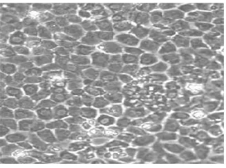
Figure 1: A surface view of a typical epithelium, displaying a regular polygonal mor-phology. Image courtesy of Martin Nelson (Wolfson Centre for Stem Cells, Tissue Engineering and Modelling; Centre for Biomolecular Science; University of Notting-ham; UK).

is derived. Solution of this model is compared to numerical simulations of the discrete system in_§4, illustrating the generation of patterns under spatial variation of feedback strength, and pattern competition and travelling-wave behaviour in the case of uniform feedback. In _§5 our findings are summarised, together with suggestions for future research.

2

Pattern formation in a discrete Delta-Notch

intercel-lular signalling model

2.1

Formulation

In Collier et al (1996), the feedback between the binding of a membrane-bound sig-nalling protein, Delta, to its receptor, Notch, and subsequent Delta expression was considered. The crucial aspect of the feedback loop is that elevated Delta expression in a cell downregulates Delta expression in its neighbours via the receptor, Notch. This mechanism, known as lateral inhibition, is a fundamental cell-fate control mechanism (Mitsiadis et al, 1999), creating fine-grained patterns in developing tissues which de-termine subsequent cell development. The key postulate of the Delta-Notch signalling model is that the level of activated Notch in a cell determines its fate: low levels lead to the adoption of default (primary) fate, whilst high levels relegate the cell to the secondary fate. In the specific case of nervous tissue in Drosophila, the primary fate corresponds to the adoption of a neural phenotype, the secondary fate being the main-tenance of the epidermal phenotype (Lehmann et al, 1983; Campos-Ortega, 1993). The model is formulated in terms of Delta and Notch “activity”; the details of the signalling pathways, as well as cell division, are neglected for simplicity.

The model comprises a pair of ordinary differential equations that govern the levels of Delta (dj) and Notch (nj) activity in each cell ( j). In dimensionless terms these are

(Collier et al, 1996):

˙

dj=λ(g(nj)−dj), (1a)

˙

nj=f(dj)−nj, (1b)

where dots denote differentiation with respect to time andλ is the ratio of the decay rates of Delta and Notch activity. We remark that a single subscript is used to denote each cell for simplicity; however, generalisation to higher spatial dimensions is trivial. In (1), f(dj)and g(nj)are feedback functions representing the coupling between

adja-cent cells and the inhibitory effect of Delta-Notch binding, respectively and djdenotes

the mean level of Delta activity in the N cells surrounding cell j:

f(σ) = σ

k

a+σk,g(σ) =

1

1+bσh, dj=

1 N

N

∑

di. (2)

The positive parameters k, h, a and b determine the feedback strength. Detail of the biological meaning of the exponents together with example molecules is given in Webb and Owen (2004).

stimulation, leading us to include spatial variation in the parameters associated with the feedback functions f and g. For constant feedback strength Collier et al (1996), Plahte (2001) and Plahte and Øyehaug (2007) remark that a striking feature of the Delta-Notch model is the robustness of the fine-grained pattern1. Webb and Owen (2004) have demonstrated that cell shape is an important factor in the patterns produced in cell-signalling models; furthermore, certain epithelial cells are not necessarily well-approximated by square cells (see Figure 1). In view of these considerations, below, we extend our previous work (O’Dea and King, 2011) to investigate the emergence of fine-grained patterning modes in hexagonal cells in response to variation in the parameters associated with the feedback strength.

2.2

Patterning and stability

By linear and bifurcation analysis we now determine the parameter regimes for which fine-grained spatial patterning will be produced by this model. In arrays of square cells, fine-grained patterning corresponds to patterns with a period of two cell lengths in each direction (and the periodic unit therefore contains four cells). In contrast, the shortest wavelength pattern which fits onto a discrete hexagonal mesh is of period three in each direction (the periodic unit containing three cells), corresponding to the dominant fine-grained patterning mode discussed in_§2.1. In each case, in what follows, we will refer to these as patterns of period two and three, respectively. Due to the local nature of the juxtacrine signalling mechanism, considering patterns of Delta and Notch activity in such a periodic unit provides insights into more extensive arrays and the results obtained are crucial to the subsequent multiscale analysis. The system (1) reduces to a system of six coupled equations to which the solutions are either homogeneous or patterned with a wavelength of three cells. We remark that, in view of (2), in the period-three regime the connectivity of the periodic network is identical both in arrays of hexagonal cells and in one-dimensional strings. For the purposes of the following patterning and stability analysis, we therefore persist with the single index j to indicate each of the three cells in the periodic unit.

Via linear analysis of (1) it is straightforward to show that the homogeneous state is unstable and period three patterns exist if f′(d∗)g′(n∗)<−2, where(n∗,d∗)are the homogeneous steady states satisfying d∗=g(n∗),n∗=f(g(n∗))and′denotes differen-tiation (Collier et al, 1996). Furthermore, the period three pattern is the fastest growing mode from the uniform state. Similarly, period three steady states n∗_j, d∗_j ( j=1,2,3) become unstable to period three perturbations if f′(d∗_j)g′(n∗_j)<−2, where d∗_jdenotes the weighted sum of neighbouring steady-state values defined by (2).

The transition from parameter regimes in which the homogeneous steady state is stable (so that adjacent cells exhibit identical levels of Notch activation and thereby attain identical cell fates) to that in which stable heterogeneous states emerge leads to the generation of fine-grained patterns of Delta and Notch upregulation (so that nearby cells diverge to different fates). We remark that since it is postulated that the level of Notch activity determines its fate, in the following, we will use the terms “up-” or “down-regulated” to refer to the level of Notch activation in each cell.

Bifurcation analysis indicates that the system admits three distinct pattern types of period three: (i) a ratio of two identically up-regulated cells to one down-regulated,

1_{Plahte (2001) suggested that the feedback structure of the model (1) fundamentally favours this pattern,}

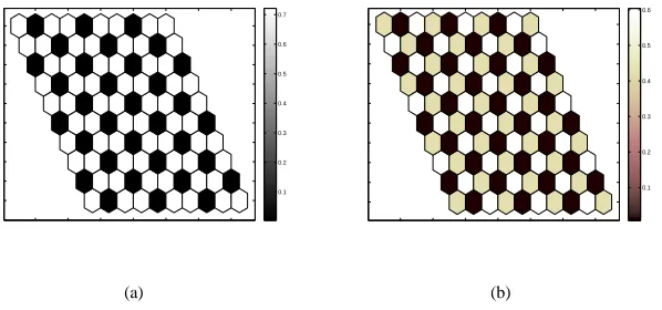
(ii) a ratio of two identically down-regulated cells to one up-regulated and (iii) one up-regulated cell, one down-regulated and one intermediate; in the following, we shall refer to these patterns as type (i), (ii) and (iii) for clarity. Figure 2 shows typical numerical simulations displaying period three patterns of type (i) and (iii).

0.1 0.2 0.3 0.4 0.5 0.6 0.7

(a)

0.1 0.2 0.3 0.4 0.5 0.6

(b)

Figure 2: Typical numerical simulations showing the level of Notch activity in a 10_×10 section of a two-dimensional periodic array of hexagonal cells illustrating the steady-state type (i) and (iii) patterning modes. Parameter values:λ=1, a=0.1, b=100 and (a) k=h=2, corresponding to type (i); (b) k=h=4.25, corresponding to type (ii).

In the three cell system under consideration the various pattern permutations mean that types (i) and (ii) comprise three patterns each, whilst type (iii) contains six pattern configurations. Figure 3 shows the transition from one patterning mode to the next under variation of the exponents k and h which govern the feedback strength in the signalling model (similar bifurcation behaviour is observed under variation of k or h alone), indicating that there is a distinct range of parameter space in which each of the three types of pattern is stable, and that type (i) and (ii) patterns are stable for a significantly larger portion of parameter space than those of type (iii). We highlight that ‘stability’ as indicated in Figure 3 refers to stability of period three patterns within the three-cell periodic unit. The various pattern configurations within each pattern type are highlighted on the relevant curves; Figures 3(b) and (c) show the configurations in detail. The solution branches indicate the level of Notch activation in each cell. For instance, in the type (i) patterning regime, referring to Figure 3(a), if the level of Notch activation in a cell follows the lower solution branch marked with circles, the remaining pair of cells follow the upper branch (marked with diamonds). Similarly, in the type (ii) regime, if the level of activation in a cell tracks the upper branch (filled circles), the remaining cells track the lower branch (marked with squares); in between these parameter ranges, type (iii) patterns are observed. Lastly, we remark that the bifurca-tion structure is significantly more complex than that associated with the generabifurca-tion of period two patterns (in each coordinate direction) in square cells (O’Dea and King (2011)). It is important to note, however, that O’Dea and King (2011) considered the specific case of checkerboard patterns, for which the analysis corresponds exactly to that in a one-dimensional string of cells. In the case for which the periodic unit con-tains four distinct levels of upregulation (only two exist for checkerboard patterns) the behaviour is likely to be more complex.

state subcritically; patterns containing three distinct levels of upregulation (type (iii) patterns) and type (ii) patterns are created at subsequent bifurcations labelledC_a–C_d. The bifurcation pointsC_a,C_candC_b,C_dform solution pairs: the Notch activity in two of the three cells diverges from the supercritical bifurcations atC_bandC_c; the remain-ing cell increases or decreases from its bifurcation point valueC_aorC_dvia the relevant solution branch. The pitchfork bifurcations atC_bandC_{cimply that patterns with three}

distinct levels of Notch activation are generated from type (i) or type (ii) patterns by the local, symmetric divergence of two of the three cells. Figure 4(a) illustrates how this bifurcation structure changes under variation of the inhibitory feedback function parameter b, demonstrating that the five bifurcations shown in Figure 3 collapse onto a single patterning bifurcation from the homogeneous steady state as b is reduced. Addi-tionally shown are the resulting pattern-forming bifurcations obtained under variation of k,h for values of b at which the bifurcations collapse onto a subcritical bifurcation (Figure 4(b)) and a supercritical pitchfork-like bifurcation (Figure 4(c)). Here, only stable type (ii) and unstable type (i) patterns exist.

0 1 2 3 4 5 6 7 8 9 10

0 0.1 0.2 0.3 0.4 0.5 0.6 0.7 0.8 0.9 1 n

k=h

n∗

(1 : 1 : 1) (−,+,−) (+,−,+) (+,−,−) (−,+,+)

(a) C_a

C_b

C_c

C_d

C∗

3.8 4 4.2 4.4 4.6 4.8 5 5.2 0.4 0.5 0.6 0.7 0.8 0.9 n

k=h

(+,−,−)

(+,−,−)

(+,+,−)∗

(+,+,−)∗

(+,−,+) (+,−,+)

(3,2, 1∗)

(3,1, 2)

(2,3,1)∗

(2,1,3) (b)

4 4.2 4.4 4.6 4.8 5 5.2 5.4 0 0.05 0.1 0.15 0.2 0.25 0.3 0.35 0.4 n

k=h

(−,+,+) (−,+,+)

(−,+,−)∗ (−,+,−)∗ (−,−,+) (−,−,+)

(1,3,2

)

∗

(1,2 ,3) (2,3,1)∗

(2,1,3) (c)

Figure 3: (a) Bifurcation diagram showing the level of Notch activation for the system (1) in a three cell system with periodic boundary conditions under variation of the parameters k and h. The stable homogeneous steady state, and various period three patterns, are identified via different line styles; the corresponding unstable states are represented by dotted lines (the unstable homogeneous state is indicated by a dot-dash line for clarity). The various solution branches indicate the level of Notch activation in each of the three cells; see text. Bifurcations at which patterns are created from the homogeneous state and between different pattern types are denotedC∗andC_a–

C_d, respectively. The homogeneous steady state is denoted n∗; for type (i) and (ii) patterns, up- and down-regulated cells are denoted ‘+’ and ‘₋’; type (iii) is denoted

(1 : 1 : 1). Panes (b) and (c) show in more detail the behaviour near the branch points

C_bandC_c at which the transition from types (i) and (ii) to type (iii) patterns occurs. The different type (iii) steady states are labelled 1,2,3 to denote increasing levels of Notch upregulation in each cell. Asterisks denote type (iii) solutions with associated type (i) or (ii) patterns.

pa-100 ₁₀1 ₁₀2 ₁₀3 0

2 4 6 8 10 12

k

=

h

b

(a) C∗

C_a,C_c

C_b,C_d

0 5 10 15 20 0.7

0.75 0.8 0.85 0.9 0.95

n

k=h

(b)

0 2 4 6 8 10 0.45

0.5 0.55 0.6 0.65 0.7 0.75 0.8 0.85 0.9 0.95

n

k=h

(c)

Figure 4: (a) Bifurcation diagram showing the positions of the bifurcation pointsC∗

andC_a,C_c–C_d (see Figure 3) under variation of the parameters b and k, h. For the particular value a=0.1 chosen here, the five bifurcations coalesce at b∗_≈1.927. Panes (b) and (c) illustrate the change in bifurcation structure for illustrative values of b at which only unstable type (i) and stable type (ii) patterns exist. In each case the upper branch indicates the steady-state values of two of the three cells and the lower branch, the remaining cell. In (b) b=1 and (c) b=b∗; solid and dotted lines indicate stable and unstable branches, respectively. The structure for b=100 is shown in Figure 3.

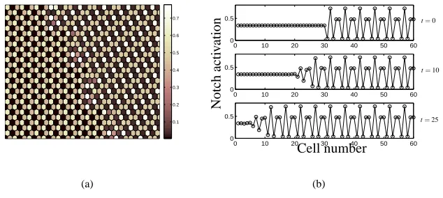
rameter values. We remark that longer-range patterns (of period greater than three) may be generated in this array of hexagonal cells by appropriate choice of periodic initial conditions and domain size. We note that these patterns are stable to periodic or ape-riodic perturbations but that their domain of attraction is small and therefore are only observed for suitable initial data. Numerical simulations of (1) indicate that regions of these longer-range patterns form stable patterned distributions when competed with period-three patterns and, additionally, are able to invade the unstable homogeneous steady-state (invasive or competitive behaviour is generated via initial data comprising a region of stable longer-range patterning adjacent to the unstable homogeneous state or stable period-three pattern in the remainder of the domain). However, the introduc-tion of random noise to periodic initial data, which is not itself a steady state of (1), seems always to result in the emergence of the dominant period-three patterning mode; similarly, an initial state comprising a region of unstable period-three pattern adjacent to a region of stable longer-range pattern, leads to the invasion of the unstable state with the corresponding stable period-three, rather than long-range, pattern (though the region of stable longer-range pattern remains). Figure 5(a) shows an illustrative stable pattern configuration obtained by competition of stable period-three and period-five patterns; Figure 5(b) shows the modulated travelling wave of period-five pattern invad-ing the unstable homogeneous state. Lastly, we note that the range of patterns formed is limited by the hexagonal mesh; in particular, patterns of even period in each coordi-nate direction are prohibited (though we remark that striped patterns of arbitrary period are, of course, permitted).

0.1 0.2 0.3 0.4 0.5 0.6 0.7

(a)

0 10 20 30 40 50 60

0 0.5

0 10 20 30 40 50 60

0 0.5

0 10 20 30 40 50 60

0 0.5

Cell number

N

o

tc

h

ac

ti

v

at

io

n t=0

t=10

t=25

(b)

Figure 5: Numerical simulations of (1) performed in a 60_×60 hexagonal mesh illus-trating the behaviour of longer-range patterns. (a) A stable configuration comprising a stable period three pattern of type (iii) (left) adjacent to a stable period five (right) Notch activation pattern. (b) The modulated wave of period-five Notch activation trav-elling through the hexagonal mesh ( j,l) and invading the unstable homogeneous steady state at successive times t=0,10,25 along the line l=30. Initial conditions comprise the domain split equally between the unstable homogeneous state ( j<30) and stable period-five pattern ( j>30). All parameter values as in Figure 2(b).

direction. In hexagonal cells, the fine-grained patterning mode corresponds to patterns of period three in each direction. Collier et al (1996) identified these patterns as the fastest-growing mode a via linear analysis. The results contained in this section show that the generation of fine-grained patterns in hexagonal cells is significantly more complex than their checkerboard counterparts in square cells. We have isolated the three possible types of fine-grained pattern, demonstrated their robustness via numeri-cal simulation and shown how the bifurcation structure varies under variation of certain feedback parameters. Such information will prove crucial for the following multiscale analyses. In addition, via numerical simulations of (1) we have shown that patterns of wavelength greater than three may be produced by this model, though these patterns have small domains of attraction and are therefore only observed for suitable initial data, further exemplifying the dominance of the fine-grained model.

In the following sections, we employ a multiscale analysis to construct continuum models of the period-three patterning behaviour for parameter values near the pattern-ing bifurcation points investigated above.

3

Multiscale analyses of Delta and Notch activity in an

array of hexagonal cells

3.1

Model formulation

of the domain, or transition from one patterning mode to the next; in the following, we construct continuum models which capture fine-grained pattern generation in re-sponse to macroscale tissue stimulation, corresponding to spatial variation in feedback strength. (Such formulations include spatially-uniform feedback as a special case, anal-ysis of which will be especially instructive when considering pattern competition and travelling-wave behaviour.) In a biological context, such parameter variation might correspond to differences in the sensitivity of the cells to Delta-Notch binding, leading to the adoption of a particular programme of gene activation by a subset of the cell population according to spatial position. Such environmental inhomogeneities are a common feature of biological systems, such as in embryonic tissue growth. We note, however, that the parameter values employed in the remainder of this work are chosen to illustrate the interesting patterning behaviour exhibited by the model and investi-gated in_§2.2 and are not motivated by specific biology.

To capture the different facets of the system (1) in the period-three regime within appropriate continuum representations, we consider in turn (a) the patterning bifurca-tion from the homogeneous state, (b) the transibifurca-tion between different period three pat-terning regimes and, (c) the behaviour for parameter values close to the set for which the separate bifurcation points collide leaving a single pitchfork bifurcation (see Fig-ures 3 and 4(a,c)). As remarked earlier, since in the parameter regime b>b∗, illustrated in Figure 3(a), the bifurcation from the homogeneous state generating type (i) patterns is sub-critical, the asymptotic behaviour derived in case (a) will not be reflected in the observed solutions to (1). However, the simple model analysed here is ideally suited to illustrate our methodology; the analysis holds for alternative signalling models whose stability properties imply that the results are more immediately applicable. To construct a continuum model capturing period three patterning phenomena in response to spatial variations in feedback strength, a homogenisation process is required. To preserve the local periodicity, we assume that the variation of the spatially non-uniform parameter is slow compared to the variations of Delta and Notch activity: that is, we construct two-scale models which capture fine-grained period-three pattering patterning phenomena. This separation of scales (between ‘fast’ and ‘slow’ variation) allows the integration of fine-grained (microscale) patterning within a macroscale framework.

j,l j+1,l j−1,l

j,l+1

j,l−1 j+1,l+1

j−1,l−1

δ

x=δj

ˇ

y=δl

ψa

ψc

ψb

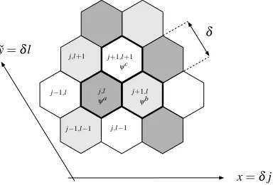
Figure 6: The discrete labelling scheme and corresponding continuum coordinates em-ployed for the multiscale analysis of pattern formation in an array of hexagonal cells. The shading indicates cells with different levels of Notch and Delta activity, in which the continuum variablesψi_{(xˇ,yˇ,t), i=a,b,c are defined. The periodic unit for the}

The continuum model is derived as follows. Considering an array of hexagonal cells, we denote the distance between cell centres byδ _≪1, introduce slowly varying continuum variables ˇx=δj, ˇy=δl and represent the levels of Delta and Notch activity in the multiple-scales form: d_j,l=d(j,l,xˇ,yˇ,t), n_j,l=n(j,l,xˇ,yˇ,t), in which j,l repre-sent the fast, and ˇx,y the slow, spatial scales. The labelling scheme for hexagonal cells,ˇ together with the periodic repeating unit for the period three pattern is illustrated in Figure 6. Additionally, since adjacent cells differ significantly in their Delta and Notch activity the patterning regimes, we write:

d(j,l,xˇ,yˇ,t) =da(xˇ,yˇ,t), n(j,l,xˇ,yˇ,t) =na(xˇ,yˇ,t): (j+l)mod3=2, (3) d(j,l,xˇ,yˇ,t) =db(xˇ,yˇ,t), n(j,l,xˇ,yˇ,t) =nb(xˇ,yˇ,t): (j+l)mod3=0, (4) d(j,l,xˇ,yˇ,t) =dc(xˇ,yˇ,t), n(j,l,xˇ,yˇ,t) =nc(xˇ,yˇ,t): (j+l)mod3=1, (5) and we will refer to the cells corresponding to equations (3)–(5) as types a–c. We remark that since the discrete labelling scheme underpins our multiscale approach, we are unable, as it stands, to accomodate cell division, which would require a global relabelling; our analysis applies on the timescale of Delta-Notch mediated cell fate determination, which is significantly exceeded by that of the cell cycle (Hartenstein & Posokony, 1990).

Transforming to an orthogonal Cartesian coordinate system(x,y) = (xˇ₋yˇ/2,√3 ˇy/2), expanding in Taylor series and exploiting the periodicity, the spatial coupling term di for each cell type i may be written:

di=1

2

∑

q6=i

dq+δ 2

8 ∇

∑

q6=i

dq+O₍δ4_), i=a,b,c. (6)

Spatial variation in biochemical or biophysical conditions within the domain (lead-ing to differences in feedback strength) is modelled by introduc(lead-ing slow spatial varia-tion to the parameters k and h. For simplicity, we assume k=h and keep the remaining parameters fixed; we assume k=h=k(x,y). We expand around the bifurcation point under consideration (C∗_, C_a–C_d; see Figures 3 and 4) via:

k(x,y;ε1) =k∗+ε1ˆk(x,y), (7)

di(x,y,t;ε2) =di∗+ε2d1i(x,y,t) +ε22d2i(x,y,t) +···, (8)

ni(x,y,t;ε2) =ni∗+ε2ni1(x,y,t) +ε22ni2(x,y,t) +···, (9)

where i=a,b,c indicates expansions associated with each cell type, k=k∗denotes the relevant bifurcation point, at which ni∗, di∗are the steady states associated with each cell type, andε1(δ),ε2(δ)≪1. Additionally, we rescale time according toτ=ε3(δ)t, whereε3(δ)≪1 will be chosen such that we analyse the equations at the timescale on which spatial coupling first appears.

We now pause to define some notation which will be of use in the following sec-tions. We define linear operatorsL andM as follows:

L₍η_,ξ_,ν_{) =g}′₍ν₎η₋ξ_,M₍η_,ξ_,ν_{) =}ξ_f′₍ν₎₋η_{, (10)}

together with the averages di_pfor each cell type i at the pthasymptotic order:

di_p=1

2_q

∑

6

=i

3.1.1 Emergence of patterns from the homogeneous steady state

In this section, we consider the generation of fine-grained patterns from the homoge-neous steady state at the bifurcation pointC∗in the regime b>b∗as illustrated in Figure 3(a). Employing the linear operators (10), the scalingsε1=ε2=ε3=δ2, the

averages (11) and noting that atC∗,(ni∗_,di∗_{) = (n}∗_,d∗_{)for i=a,b,c, the equations}

governing Delta activity in each cell type i at each order are:

O_{(1): 0=g(n}∗_)−d∗_{, (12)}

O₍δ2_{): 0=}L_(ni

1,d1i,n∗) +F1(n∗), (13)

O₍δ4₎: 1

λ∂

d₁i

∂τ =L(ni2,d2i,n∗) +

g′′(n∗)(ni₁)2

2 +G1(n

∗_)ni

1+F2(n∗),

(14)

and Notch is governed by:

O_{(1): 0=f(d}∗_)−n∗_{, (15)}

O₍δ2₎: 0=Mni₁,di₁,d∗+_Fˆ_1(d∗_{), (16)}

O₍δ4₎:∂n

i

1

∂τ =M

ni₂,di₂,d∗+(d

i

1)2

2 f

′′_(d∗_{) +G}ˆ_1(d∗_)di

1+Fˆ2(d∗) +

f′(d∗)

4 ∇

2_di 1.

(17)

The functions Fp, ˆFp and Gp, ˆGp are the O(δ2p)perturbations to g, f and g′, f′,

expanded around the bifurcation point value k∗, and defined by:

Fp=ˆk∂ p_g

∂np,Fˆp=ˆk

∂p_f

∂dp,G1=ˆk

∂2_g

∂n∂h, Gˆ1=ˆk

∂2_f

∂d∂k, (18) these being evaluated at k=h=k∗, d=d∗and n=n∗, and in view of the expansion (7) depend on the spatial coordinates x and y.

TheO₍δ2_{)linear system is of rank four and therefore has two levels of degeneracy,}

reflecting the additional degree of freedom implied by the analysis of a periodic unit of three cells (in comparison to that observed when analysing checkerboard patterns) in which the different cell types may be freely interchanged. Noting that f′(d∗)g′(n∗) =

−2 (see_§2.2) and ni∗=n∗for i=a,b,c, the combinations:

g′(n∗)M_ni

p,d i p,d∗

−g′(n∗)M_na

p,d a p,d∗

+L _ni

p,dip,n∗

−L _na

p,dap,n∗

, (19)

where i=b,c and p=1,2, . . ., are identically zero. These correspond to the two eigen-vectors (with zero eigenvalue) of the linear system, based on which we make the ansatz:

  d1 D1 e d1 

=A(x,τ)

 − 1 0 1 

+B(x,τ)

 − 1 1 0 

+C(x,t), (20)

where A and B are to be determined and, from (13), (16) we obtain:

C= g′(n∗)_Fˆ_1(d∗_{) +F1(n}∗_{)/3. We remark that through appropriate choice of A, B,}

Employing the linear combinations (19) to eliminate theO₍δ2_{)perturbations n}i

2,

di

2, equations (12)–(17) may be expressed as the following pair of coupled partial

dif-ferential equations for A(x,τ), B(x,τ):

Λ∂η

∂τ (A+2B) =α1 4γB+2γA−2AB−A2

+ β1+∇2

(A+2B), (21)

Λ ∂

∂τ(2A+B) =α1 4γA+2γB−2AB−B2

+ β1+∇2

(2A+B), (22) whereΛ,γ,α1andβ1are defined by:

Λ=4(λ+1)

λ , γ=g′(n∗)Fˆ1(d∗) +F1(n∗), α1=

g′(n∗)f′′(d∗)

2 +

2g′′(n∗) [g′_(n∗_)]2, (23)

β1=

4G1(n∗)

g′_(n∗₎ −2g′(n∗)Gˆ1(d∗)−

4g′′(n∗)F1(n∗) [g′_(n∗_)]2 −g

′_(n∗_)f′′_(d∗_{)γ. (24)}

We reiterate that, in view of equations (7) and (18),γ=γ(x,y)andβ1=β1(x,y), while

Λandα1are constants. The corresponding Notch activity is given by equation (13).

As in the case of square cells (see O’Dea and King (2011)), equations (21) and (22) demonstrate that, on the macroscale, the juxtacrine signalling interaction manifests it-self as linear diffusion, with effective diffusivity 1/Λ, despite the short-range patterning under consideration.

This continuum model differs from that derived in O’Dea and King (2011) (in which a checkerboard patterning regime in square cells was considered) by the quadratic (rather than cubic) form of the nonlinearity, due to the asymptotic scalings appropriate to reflect the solution behaviour nearC∗_{. Additionally, we have expressed our}

equa-tions in a more general form to enable the wider array of period three modes to be captured.

We note that the form of the continuum model is not crucially dependent on the details of the underlying signalling system; additional interaction terms (such as those of the form njdjor njdjas employed by Owen and Sherratt (1998) in a more complex

juxtacrine signalling model, accommodating ligand, free receptors and bound recep-tors) do not materially affect the diffusive interaction or the quadratic nonlinearity. As noted above, since the bifurcation atC∗is subcritical, the behaviour captured by equa-tions (21) and (22) will not be reflected in the observed solution behaviour; however, the analysis presented here will apply to similar systems whose stability does not con-form to that shown in Figure 3. For constant parameter values, the unicon-form steady states of (21) and (22) are determined by solving a pair of coupled quadratic equa-tions. (We highlight that these are “uniform” in the sense that they are constant for their associated cell type, adjacent cells attaining different steady states.) The signs and magnitudes of the parametersγ, α1andβ1in (21), (22) determine the existence

of such solutions, reflecting the stability properties of the underlying discrete system. In the case investigated here, multiple steady-state solutions to (21), (22) exist on both sides of the bifurcation point, reflecting its inability to differentiate between stable and unstable states; in contrast, a supercritical transition, such as the pitchfork bifurcations atC_b,C_{c, would imply a reduction in the number of real steady states as the bifurcation}

point is traversed.

3.1.2 Transitions between patterned states

C_d, as illustrated in Figure 3. We note that, in contrast to the subcritical behaviour analysed in _§3.1.1, in this case, the transitions occur at supercritical pitchfork-type bifurcations; the continuum model we shall derive is therefore immediately applicable to the dynamics of the underlying discrete system.

Adopting the notation employed in_§3.1.1, the appropriate linear combinations in this case are:

g′(ni∗)M_ni

p,d i p,d

i∗

−g′(na∗)M_na

p,d a p,d

a∗

+L _ni

p,dip,ni∗

−L _na

p,dap,na∗

,

(25) wherein i=b,c and ni∗, di∗now denote the levels of Notch and Delta activity in each cell type at the bifurcation point between pattern types, again denoted k∗in each case.

Considering the bifurcation pointsC_b,C_d at which the pattern has a ratio of two upregulated cells to one downregulated cell (see Figure 3), it may be observed that the downregulated state is an order of magnitude smaller than the upregulated state and we therefore scale the downregulated state withδ. Figure 3 indicates that at the bifurca-tionsC_a,C_{c, the steady states of Notch activity are of comparable order; however, the}

corresponding up- and downregulated steady states of Delta activity display an order of magnitude disparity (not shown) and a corresponding rescaling must therefore be chosen when considering these bifurcations. We remark that this change in scalings is also revealed from the asymptotic analysis.

In the more general case for which the downregulated steady-state value of Notch activation is of the same order as the level of upregulation, the scaling employed in

§3.1.1 is appropriate. Considering a bifurcation of the formC_b,C_d(with steady states of comparable order), the calculation follows the same method as that outlined in_§3.1.1 and we obtain:

Λ ∂

∂τ(A+2B) =α1 4γB+2γA−2AB−A2

+ β1+∇2

(A+2B), (26)

Λ ∂

∂τ(2A+B) =αA2+βB2+κAB+µA+νB+χ+∇2(2A+B), (27)

in whichΛ,α1,γandβ1are defined by (23), (24) but evaluated at the new bifurcation

point k∗, na∗, da∗(corresponding to the upregulated Notch activation state). We remark that, since in the case under consideration both cells of type a and b are in the upregu-lated state, da∗=db∗= (da∗_+dc∗_{)/2, d}c∗_=da∗_{. Application of the linear combination}

(19) therefore results in the PDEs (26) and (21) having identical form. The parameters

α–χ are known functions of both up- and down-regulated steady states: ni∗, di∗, di∗ (i=a,c), but are too cumbersome to include here; these are included in Appendix A for completeness.

We now consider in detail the behaviour atC_b,C_{dunder the configuration}

(na∗,na∗,nc∗), where nc∗=δnˆc∗ and the steady-states na∗and ˆnc∗ areO_{(1). In this}

case, at first order, the level of Notch activation in cells of type a and b diverges at the pitchfork bifurcationC_{b, the activity in type c cells remaining constant. Such}

be-haviour corresponds to choosing A=0 in equation (20). Here, the appropriate scaling isε1=ε3=δ2andε2=δ so that spatial and temporal variation enters atO(δ3). The

remaining two configurations obtained under cyclic permutation may be analysed in a similar way and correspond to B=0 and A=₋B in equation (20) in each case. We note that an equivalent derivation provides an equation governing the transition between pattern types (ii) and (iii) atC_a,C_c, but is omitted.

equa-tions governing Notch and Delta activity in each cell type are as follows:

O₍1): 0=g(ni∗)₋di∗, 0=f(di∗)₋ni∗ (28)

O₍δ_{): 0=}L_(ni

1,di1,ni∗), 0=M(ni1,d

i

1,d

i∗

), (29)

O₍δ2₎: 0=L₍n₂i,di₂,ni∗) +g

′′_(n∗_{) n}i

1

2

2 +F1(n

i∗_{), (30)}

0=M_(ni

2,d

i

2,d

i∗

) +f

′′_(di∗_)(di

1)2

2 +Fˆ1(d

i∗

), (31)

O₍δ3_): 1

λ ∂di

1

∂τ =L(ni3,d3i,ni∗) +ni1ni2g′′(ni∗) +

1 6g

′′′_(ni∗_)(ni

1)3+ni1G1(ni∗), (32)

∂n1

∂τ =M(ni3,d

i

3,d

i∗

) +di₁di₂f′′(di∗) +1

6f

′′′_(di∗_)(di

1)3 +di₁Gˆ1(di∗) +f′(d

i∗

)

3 ∇

2_di

1, (33)

wherein i=a,b,c and F1, Fˆ1, G1and ˆG1are defined by (18) and are evaluated at the

appropriate bifurcation point.

Employing the ansatz (20), equations (29) yield C=0. TheO₍δ3_{)equations (32),}

(33) may be reduced to a reaction-diffusion equation for B(x,t)as follows. The linear combination (25) with i=b allows removal ofO₍δ3₎perturbations, ni₃, d₃i, while

O₍δ2₎perturbations are eliminated in favour of those ofO₍δ₎via equations (30), (31) and the linear combination (25) with i=c. Lastly, we employ equation (29) to express the equation in terms of B only, obtaining:

Λ∂B

∂τ =α2B3+β2B+∇2B, (34)

whereΛis defined by equation (23) andα2andβ2(x,y)are defined:

α2=

2g′′′(na∗)

3[g′_(na∗_)]3−

g′(na∗)f′′′(da∗)

12 −

h

g′(na∗)f′′(da∗)i2

8

+α1

8

g′(na∗)f′′(da∗)

4 −

g′′(na∗) [g′_(na∗_)]2

!

, (35)

β2=

4G1(na∗)

g′_(na∗₎ −[g′(n

a∗_)]2_f′′_(da∗_)Fˆ_1(da∗_)−2g′_(na∗_)Gˆ_1(da∗₎

+α1 Fˆ1(d

a∗

)+f′(d

a∗

)F1(na∗)

2

!

. (36)

Equation (34) is invariant under the transformation B_{→ −}B, reflecting the sym-metric divergence of activity in cells of type a and b at the supercritical pitchfork bi-furcation C_{b; the level of activity in cells of type c remains constant at}O₍δ_{). The}

For constant β2 (i.e. ˆk=constant), the uniform steady states of (34) are B= (0,_±p₋β2/α2); ‘uniform’ here means that they are spatially-constant in cells of type

a. For k<k∗we findβ2>0 and only the trivial solution B=0 exists, corresponding

to the maintenance of the type (i) heterogeneous steady state: the periodic unit remains in the state n_∼(na∗,na∗,δnc∗). As the feedback strength increases,β2changes sign:

k>k∗,β260; in this regime non-trivial roots exist and the behaviour in the periodic

unit is n_∼(na∗,na∗,0) +δ(_±p₋β2/α2,∓

p

−β2/α2,nˆc∗)corresponding to the

emer-gence of type (iii) patterns. Considering only the local value of the feedback strength

β2=β2(x,y), we therefore expect the generation of patterned states to reflect the

pitch-fork bifurcation at k∗. For brevity, hereafter we will refer to this patterning behaviour as that influenced by “local feedback strength”.

We note that a similar analysis may be performed at the bifurcation pointsC_a,C_c

yielding a corresponding result.

3.1.3 Two parameter expansion

The above multiscale analyses have produced continuum models, based upon an un-derlying discrete patterning system, for the emergence of (unstable) patterns from the homogeneous steady state (_§3.1.1) and the (stable) transitions between patterns of types (i) and (ii) and types (ii) and (iii) (_§3.1.2) in parameter regimes for which these pattern-ing bifurcations are widely spaced.

Inspection of the model equations derived in_§§3.1.1 and 3.1.2 reveals that the gen-eration of, and transition between, period-three patterns is dependent onα1(for clarity,

we emphasise thatα1=α1(na∗,da∗,k∗,b), na∗and da∗being the steady states in cells

of type a at the bifurcation point k∗for a specific value of b). The multiscale anal-yses presented in_§§3.1.1 and 3.1.2 correspond to the bifurcation structure illustrated in Figure 3 for whichα1>O(1). In the caseα1=0 (b≈1.927), the five

bifurca-tions collapse onto one pitchfork-like patterning bifurcation generating stable type (ii) and unstable type (i) patterns from the homogeneous steady state (see Figure 4(c)). Here, we analyse the behaviour near the bifurcation atα1=0; inspired by Figure 4 we

consider:

b(x,y;ε4) =b∗+ε4ˆb(x,y) (37)

in addition to the expansions (7)–(9), in which(di∗_,ni∗_{) = (d}∗_,n∗_{)denote the}

homo-geneous steady-state values of Delta and Notch activity at b∗, k∗, the bifurcation point values at whichα1=0.

In this regime, the model (21) and (22) breaks down, providing only the trivial steady state; instead, a continuum model for period three patterns being generated from the homogeneous steady state is obtained by choosingε1=ε3=ε4=δ2andε2=δ

and spatial and temporal variation enters atO₍δ3_{)as in§3.1.2. The equations at each}

order are identical to (28)–(33) with f and its derivatives evaluated at di∗=d∗; here, F1, ˆF1, G1, ˆG1are theO(δ2)perturbations to f , g and f′, g′expanded around b∗, k∗.

As in the previous analysis of pattern emergence from the homogeneous steady state, the linear combinations (19) enable elimination ofO₍δ3₎perturbations (ni₃, di₃) from (32) and (33). Equations (31) allow O₍δ2₎ perturbations to be removed from the resulting pair of equations in favour of those ofO₍δ_{); employing the ansatz (20)}

differential equations for A(x,τ), B(x,τ):

λ_∂τ∂ (A+2B) =α2 A3+3A2B+3AB2+2B3

+ β2+∇2

(A+2B), (38)

λ ∂

∂τ(2A+B) =α2 B3+3A2B+3AB2+2A3

+ β2+∇2

(2A+B), (39)

whereα2andβ2are defined by (36) and evaluated atα1=0, d

a∗

=d∗. The corre-sponding Notch activity is given by equation (13).

The analyses presented in_§§3.1.1 and 3.1.2 describe the behaviour near the indi-vidual bifurcation pointsC∗ _orC_a–C_{d; above, via the isolation of the combination}

α1which dictates the bifurcation structure of the system (except in the special case

for which the downregulation of Notch activity in one cell is extreme), we have de-rived a more general formulation which captures the generation of the five bifurcation points illustrated in Figure 3. Furthermore, the model corresponding to the structure illustrated in Figure 4(c) may be recovered by setting ˆb=0.

We remark that the nonlinearities in the model (38), (39) are of a different form to those in the models (21), (22) and (26), (27), obtained by analysing pattern generation in the regimeα1>O(1)for steady states of comparable order. However, by

consider-ing the matchconsider-ing between the inner (in parameter space) formulation (38) and (39) and the outer formulations (21), (22) and (26), (27)2, it can be shown that these models are consistent in the limits ˆb_→∞, b_→b∗. This calculation is summarised in Appendix B for completeness.

3.1.4 Summary

We have employed a multiscale analysis to derive continuum models based upon the discrete Delta-Notch signalling model that describe both the emergence of period three patterns from the homogeneous steady state and the transition between two types of period-three pattern in appropriate parameter regimes.

In the former case, the bifurcation from the homogeneous state generating type (i) patterns is sub-critical, and so the asymptotic behaviour derived will not be reflected in the observed solutions to (1). However, the analysis contained herein serves to il-lustrate our methodology; similar continuum models may be derived for alternative signalling systems whose stability properties imply that the results are more immedi-ately applicable. On considering the transition between patterned states, two distinct regimes were identified. In the case for which the heterogeneous steady states of Delta and Notch activation are of comparable order, the generation of patterns from the ho-mogeneous state and the transition between patterning modes are governed by models of a similar form. In each case we obtain a pair of coupled reaction-diffusion equations with quadratic nonlinearity: equations (21), (22), (26) and (27). This deviates from the equation derived in O’Dea and King (2011), in which a cubic nonlinearity is obtained. This disparity is due to the asymptotic scalings required to capture solution behaviour near the bifurcation points in the multiscale analysis. An exception is the transition be-tween patterning modes in parameter regimes for which the downregulation in one of the three cells is extreme (the transition at the pitchfork bifurcationsC_aorC_dshown in Figure 3). Here, since the level of activation in the downregulated cell remains constant (to first order), the resulting continuum model (34) is identical in form to that derived

2_{We note that the outer pattern transition model (34) is not applicable at the edge of the inner layer since}

in O’Dea and King (2011) in which the symmetric divergence of a periodic unit of two cells at a pitchfork bifurcation was considered.

The model equations (21), (22) and (26), (27) are expressed in a more general form than that in O’Dea and King (2011), leading to a system of PDEs in place of the single PDE obtained in O’Dea and King (2011). This reflects the more complex pattern form-ing behaviour exhibited in a hexagonal mesh. In the case of checkerboard patterns, the pattern-forming bifurcation is of pitchfork type and the possible pattern configurations are equivalent up to a phase shift of a single cell. The asymptotic behaviour is therefore captured by one PDE (with cubic nonlinearity) and the Notch activation in alternate cells (n1, n2, say) diverges symmetrically from the bifurcation point; the alternative

pattern therefore displays the corresponding, but inverse, behaviour, viz: _±n1=∓n2.

In the case of patterns of period three, the various pattern configurations associated with each mode mean that such a symmetry is not sufficient to capture the entire be-haviour. A second PDE is required to provide an additional degree of freedom and these patterns may then be captured via suitable choice of the slowly-varying functions A and B. In (34), however, due to the specifics of the problem at hand, we are led to consider the case for which A=C=0 and the resulting single equation models the transition from type (i) patterns in the configuration (na∗_,na∗_,δnˆc∗_{) to corresponding}

patterns of type (iii) only. The return to a single PDE and cubic nonlinearity obtained in this case reflects that the third cell in the periodic unit remains constant to first or-der, the remaining two cells diverging symmetrically, as is the case for checkerboard patterns.

Figure 4 reveals that the bifurcation structure is controlled by the feedback parame-ter b, reflected in the appearance of the combinationα1in the asymptotic analysis; the

five bifurcations illustrated in Figure 3 collapse onto a single supercritical pitchfork-like bifurcation at a critical value b∗(corresponding toα1=0). Inspired by this, we

performed a two-parameter expansion, constructing a continuum model for the unfold-ing bifurcation at k∗, b∗. In this case, the second order equations become degenerate and the resulting reaction-diffusion equation has a cubic nonlinearity as in O’Dea and King (2011), reflecting that the behaviour in two of the three cells is identical, track-ing the upper solution branch of the pitchfork. The remaintrack-ing cell follows the lower branch; the alternative patterns are obtained by inverting this behaviour. However, a system of PDEs is nevertheless obtained, reflecting the additional possible pattern configurations. By considering matching between this formulation and the preceding analyses in appropriate limits, we confirmed that the various continuum limits are con-sistent and that the model derived for the behaviour near b∗contains the other models as limit cases.

4

Numerical results

4.1

Steady states

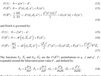
As noted above, the continuum model (21), (22) is unable to predict the observed be-haviour of the discrete model (1) since the period three patterns branch subcritically from the homogeneous steady state atC_{. In place of time-dependent numerical}

sim-ulations of (1), we therefore compare the unstable steady states of (1) nearC _with

behaviour of the nonlinear model (1) as the parameter k is varied; Figure 7(b) shows this in more detail. Clearly, the steady states of the continuum model form a good approximation to the (unstable) underlying discrete behaviour close to the bifurcation point; further from the bifurcation point, the transcritical-type behaviour predicted by the continuum limit diverges from the nonlinear model.

1.4 1.5 1.6 1.7 1.8 1.9 2 0.14

0.16 0.18 0.2 0.22 0.24 0.26 0.28

0.3 Asymptotic approximation

n

k=h

(a)

1.67 1.68 1.69 1.7 1.71 1.72 1.73 1.74 0.206

0.208 0.21 0.212 0.214 0.216 0.218 0.22 0.222 0.224

0.226 Asymptotic approximation

n

k=h

(b)

Figure 7: (a) Comparison of the steady states of Notch activity of the nonlinear system (1) near the bifurcation pointC _{(see Figure 3) with those of the continuum}

approxima-tion (21), (22); (b) the comparison in more detail. The stable steady state is indicated by a solid line, unstable nonlinear steady states by dotted lines. Parameter values as in Figure 2 except k=h as indicated.

4.2

Simulations

To illustrate the dynamic behaviour of our continuum formulations, we now present nu-merical solutions of (34) on the domain 06x6L, 06y6L and compare these to cor-responding numerical simulations of the discrete system (1). These simulations capture the transition between type (i) and type (iii) patterns. We choose ˆk(x,y) =2x/L₋1 to demonstrate how spatial variation in feedback strength dictates the emergence of fine-grained patterning in the domain. As noted in_§3.1.2, the uniform steady steady states of (34) are (0,_±p₋β2/α2). Considering only the local value of the feedback strength

β2=β2(x,y), we therefore expect the generation of patterned states to reflect the

pitch-fork bifurcation at k∗. In addition to the comparison with the underlying discrete model, in the following, we demonstrate how solutions to (34) with spatially-varying feedback differ from the pitchfork bifurcation behaviour that arises from considering only this ‘local feedback’ strength. Simulations of (38) and (39) capture the emergence of stable type (ii) patterns from the homogeneous steady state; while the specifics of the pattern transition represented by (38) and (39) are significantly different to those described by (34), the behaviour of the relevant variables at first order is qualitatively similar (two of the cells following the upper solution branch of the pitchfork-like bifurcation, the third cell tracking the lower) and simulations are therefore omitted for brevity.

Equation (34) was solved by discretising on a uniform spatial grid and employing the initial value problem solver ode15s _{in MATLAB; in the following simulations}

since the cell-scale variation has been systematically averaged out. Since we expect macroscale variation over the domain due to the chosen form of ˆk(x,y), we impose no-flux conditions at x=0,L in place of a macroscale periodic domain imposed in the discrete simulations shown in Figure 2.

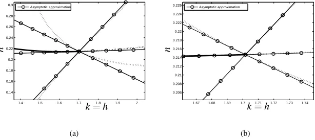
In Figure 8(a), the steady-state pattern in a 19_×19 section of a small 2D array of hexagonal cells is shown, obtained from simulation of the discrete system (1) indicating the transition from one patterning mode to the next. So that patterning effects are evident on this small domain, we chooseδ=0.5, L=10.5. In Figure 8(b) the steady-state value of the level of Notch activation in cells of type a and b as predicted by (34) are compared to a corresponding simulations of (1) in an array of 900_×900 hexagonal cells (L=9,δ =0.01), demonstrating that a smooth transition to from type (i) to type (iii) patterning is obtained. In contrast, considering only the local feedback strength (see _§3.1.2) predicts a pitchfork bifurcation from spatial homogeneity to patterning; far from the bifurcation k∗, the local feedback approximation shows good quantitative agreement with the numerical simulations.

0.1 0.2 0.3 0.4 0.5 0.6 0.7 0.8 0.9

(a)

0 1 2 3 4 5 6 7 8 9

0.15 0.152 0.154 0.156 0.158 0.16 0.162

Local feedback Type A cells

Type B cells Discrete

x

d

(b)

Figure 8: (a) The steady state level of Delta activity predicted by the discrete model (1) in a section of a two-dimensional array (δ =0.5, L=10.5), and (b) a comparison between the levels of Delta activity indicated by the discrete and homogenised models in an array of 900_×900 cells (δ =0.01, L=9) along the line y=4.5. The dotted line indicates the pitchfork transition arising from considering ‘local feedback’ (see text) only. ˆk(x,y) =2x/L₋1,∆x=1_×10−4=∆y, other parameters as in Figure 2.

4.3

Pattern invasion

4.3.1 Travelling waves