An extension of geographically weighted regression with flexible bandwidths

REGRESSION WITH FLEXIBLE BANDWIDTHS

Wenbai Yang

A Thesis Submitted for the Degree of PhD at the

University of St Andrews

2014

Full metadata for this item is available in St Andrews Research Repository

at:

http://research-repository.st-andrews.ac.uk/

Please use this identifier to cite or link to this item: http://hdl.handle.net/10023/7052

An Extension of Geographically Weighted

Regression with Flexible Bandwidths

Wenbai Yang

Supervisor: Professor A. Stewart Fotheringham

This thesis is submitted in fulfilment for the degree of PhD

at the

University of St Andrews

1. Candidate’s declarations:

I, Wenbai Yang, hereby certify that this thesis, which is approximately 37,370 words in length, has been written by me, that it is the record of work carried out by me and that it has not been submitted in any previous application for a higher degree.

I was admitted as a research student in October, 2011 and as a candidate for the degree of PhD in October, 2011; the higher study for which this is a record was carried out in the University of St Andrews between 2011 and 2014.

Date ……… signature of candidate ………

2. Supervisor’s declaration:

I hereby certify that the candidate has fulfilled the conditions of the Resolution and Regulations appropriate for the degree of PhD in the University of St Andrews and that the candidate is qualified to submit this thesis in application for that degree.

Date ……… signature of supervisor ………

3. Permission for electronic publication:

In submitting this thesis to the University of St Andrews I understand that I am giving permission for it to be made available for use in accordance with the regulations of the University Library for the time being in force, subject to any copyright vested in the work not being affected thereby. I also understand that the title and the abstract will be published, and that a copy of the work may be made and supplied to any bona fide library or research worker, that my thesis will be electronically accessible for personal or research use unless exempt by award of an embargo as requested below, and that the library has the right to migrate my thesis into new electronic forms as required to ensure continued access to the thesis. I have obtained any third-party copyright permissions that may be required in order to allow such access and migration, or have requested the appropriate embargo below.

The following is an agreed request by candidate and supervisor regarding the electronic publication of this thesis:

Embargo on both all of printed copy and electronic copy for the same fixed period of two years on the following ground: publication would preclude future publication.

Abstract

Various statistical methods have been developed for local spatial analysis. Among them Geographically Weighted Regression (GWR) is a simple yet powerful method to explore spatially varying relationships between variables. This thesis examines how GWR can be extended to investigate spatially varying relationships at various geographical scales within one model.

GWR assumes that observations near to a regression location have more influence on the estimation of local regression coefficients than do observations farther away. A single bandwidth is employed in basic GWR to control the rate of distance-decay in this influence. The magnitude of the bandwidth affects the scale of variation in the estimated regression coefficients and thus usefully reflects the appropriate spatial scale at which the processes being modelled operate. A small bandwidth suggests the processes operate over a local spatial scale, whilst a large bandwidth indicates a more regional process.

In practice, a single bandwidth as in basic GWR may not be sufficient to reflect the potentially complex spatial variations in relationships between variables in a multivariate spatial model. Therefore, in order to estimate coefficient surfaces that may vary at different spatial scales for different variables, Flexible Bandwidth GWR (FBGWR) is proposed to allow different bandwidths to be individually specified for each independent variable in a regression framework. An algorithm based on back-fitting is developed to calibrate the FBGWR model.

Dedicated to my parents for their never ending love and support. 谨以此文献给我敬爱的父母，感谢他们无尽的关爱与支持。

Acknowledgements

I have been extremely fortunate that my PhD spanned two universities: the National University of Ireland Maynooth (NUIM) and the University of St Andrews. I owe my deepest gratitude to so many people without whose guidance, advice, encouragement and support I could not have completed the work presented in this thesis.

First and foremost, I would like to express my sincere thanks to my supervisor, Professor A. Stewart Fotheringham for the knowledge, guidance and encouragement he provided throughout my PhD. It has been a great honour to have him as my supervisor. I am extremely grateful to Dr. Paul Harris, whose generous support, advice and encouragement has greatly contributed to my PhD experience. Thanks also to Professor Chris Brunsdon for his insightful suggestions during the early stages of my research.

I wish to thank Dr. Urška Demšar for her help during the transfer from Maynooth to St. Andrews and for her encouragement throughout my thesis. Thanks to Panagiota Spanou for taking care of everything I needed help with, my officemate Sila for all of the insightful discussions and encouragement that helped me through the hard times of my PhD and David in the next office for keeping me company through those late working nights.

I am grateful to everyone in the National Centre for Geocomputation, NUIM for making my time there a memorable experience. Special thanks to Dr. Jan Rigby for her advice on both a personal and academic level when acting as my PhD programme coordinator. Thanks to all of the administrative staff, especially Ann-Marie Burke and Melina Lawless for making my daily life much easier. Thanks to all of my fellow PhD students especially Conor, Binbin and Ishwari for their friendship. Thanks to all academic staff and post-docs for providing me with an inspiring work environment. I also wish to extend my thanks to Dr. Chris Lloyd from University of Liverpool and Dr. Jed Long for examining my thesis.

Funding

Research presented in this paper was funded by a Strategic Research Cluster grant (07/SRC/I1168) by Science Foundation Ireland under the National Development Plan. Additional funding was provided by the University of St Andrews as part of Professor A. Stewart Fotheringham’s start up grant. Partial funding by the Chief Scientist Office

I

Contents

Chapter 1 Introduction ... 1

1.1 General overview ... 1

1.2 Research objectives ... 3

1.3 Thesis structure ... 3

Chapter 2 Spatial analysis and spatial regression models ... 5

2.1 Spatial analysis in general ... 5

2.1.1 Quantitative geography ... 6

2.1.2 Spatial econometrics ... 7

2.1.3 Statistics ... 7

2.2 Spatial issues in spatial modelling ... 8

2.2.1 Spatial dependence ... 8

2.2.2 Spatial heterogeneity ... 9

2.2.3 Interaction between spatial autocorrelation and spatial non-stationarity 10 2.3 Non-spatial regression models ... 10

2.3.1 Standard regression ... 10

2.3.2 Local regression ... 11

2.3.3 Generalized additive model ... 13

2.4 Spatial regression models ... 15

2.4.1 Global methods ... 15

2.4.2 Local methods ... 17

2.5 Summary ... 23

Chapter 3 Geographically Weighted Regression... 25

3.1 Basic methodology ... 25

II

3.3 Software for GWR ... 32

3.4 Alternative versions of GWR ... 33

3.5 Extensions of GWR ... 34

3.5.1 Mixed GWR ... 34

3.5.2 Generalized GWR ... 35

3.5.3 Robust GWR ... 36

3.5.4 Penalized GWR ... 36

3.5.5 Other Extensions ... 37

Chapter 4 Flexible Bandwidth GWR ... 38

4.1 Why Flexible Bandwidths ... 38

4.2 Basic methodology ... 39

4.3 Back-fitting algorithm ... 40

4.4 Bandwidth selection ... 42

4.4.1 Bandwidth selection for basic GWR ... 42

4.4.2 Bandwidth selection for FBGWR ... 44

4.5 Algorithm development ... 45

4.5.1 Choice of initial guesses ... 46

4.5.2 Choice of termination criterion ... 47

Chapter 5 Experiment on synthetic datasets ... 49

5.1 Experimental design ... 49

5.1.1 Simulation study ... 49

5.1.2 Dataset design ... 50

5.1.3 Model evaluation ... 54

5.1.4 Experiment environment ... 54

5.2 Bandwidth selection ... 55

5.2.1 Bandwidth optimization by brute force ... 55

III

5.2.3 Bandwidth optimization synchronously ... 61

5.3 Choice of initial guesses ... 70

5.3.1 Bandwidths selected ... 72

5.3.2 Estimated coefficients ... 73

5.3.3 Algorithm efficiency ... 75

5.4 Choice of termination threshold ... 76

5.5 Flexible bandwidths in scenarios ... 78

5.5.1 Scenario 1: high heterogeneity β1 + high heterogeneity β2 ... 80

5.5.2 Scenario 2: low heterogeneity β1 + low heterogeneity β2 ... 87

5.5.3 Scenario 3: zero heterogeneity β1 + low heterogeneity β2 ... 93

5.5.4 Scenario 4: high heterogeneity β1 + zero heterogeneity β2 ... 96

5.5.5 Scenario 5: high heterogeneity β1 + low heterogeneity β2 ... 100

5.6 Summary ... 103

Chapter 6 Case study on Irish Famine ... 105

6.1 Irish Famine data ... 105

6.1.1 Irish Famine ... 105

6.1.2 Data source ... 105

6.1.3 Data preparation ... 108

6.2 Model building ... 111

6.2.1 Global model ... 111

6.2.2 Basic GWR ... 112

6.2.3 FBGWR with auto-selected bandwidths ... 115

6.2.4 FBGWR with a priori bandwidths ... 118

6.2.5 Mixed GWR ... 118

6.3 Model comparison ... 119

6.4 Collinearity diagnostic ... 121

IV

6.6 Summary ... 132

Chapter 7 Conclusions ... 135

7.1 Research achievements ... 135

7.2 Applicability of FBGWR ... 136

7.3 Future directions ... 137

7.3.1 Limitations ... 137

7.3.2 Future work ... 137

7.4 Final remarks ... 138

V

List of Figures

Figure 3-1 A typical weighting function ... 27

Figure 5-1 A grid for generating the simulation dataset ... 50

Figure 5-2 Illustration of the data generating process (2D) ... 52

Figure 5-3 Illustration of the data generating process (3D) ... 53

Figure 5-4 Surfaces of the true coefficients ... 56

Figure 5-5 Scatterplot of total AIC score against various bandwidths ... 58

Figure 5-6 Surface of residuals (left) and the normal Q-Q plot (right) ... 59

Figure 5-7 Scatterplot of total AIC score against various bandwidths ... 60

Figure 5-8 Procedure of iterative bandwidth selection through back-fitting ... 61

Figure 5-9 Updates of bandwidths selected during back-fitting ... 62

Figure 5-10 Updates of bandwidths selected during back-fitting (with X1 and X2 swapped in the model) ... 63

Figure 5-11 Convergence of the back-fitting processs ... 64

Figure 5-12 An example of nonconvergent back-fitting... 65

Figure 5-13 Updates of bandwidths during a nonconvergent back-fitting ... 65

Figure 5-14 Convergence after remedy on a nonconvergent example ... 66

Figure 5-15 Examples of nonconvergent back-fitting ... 68

Figure 5-16 Examples of selecting steady bandwidths automatically ... 69

Figure 5-17 An example of selecting steady bandwidths manually (the plot on the left has been zoomed in and trimmed to show more details) ... 69

Figure 5-18 A second example of selecting steady bandwidths manually (the plot on the left has been zoomed in and trimmed to show more details) ... 70

Figure 5-19 Surfaces of the true coefficients ... 72

Figure 5-20 Bandwidths selected by GWR and FBGWR with different initial guesses ... 73

Figure 5-21 Estimated coefficient surfaces from GWR and FBGWR with different initial guesses ... 75

Figure 5-22 Iterations and time cost in FBGWR with different initial guesses... 75

Figure 5-23 Iterations required in FBGWR with different termination thresholds ... 77

VI

Figure 5-25 Surfaces of the simulation coefficients ... 79

Figure 5-26 Bandwidths selected in 10 simulations ... 80

Figure 5-27 RMSEs of estimates in 10 simulations ... 81

Figure 5-28 Estimated coefficient surfaces from basic GWR and FBGWR ... 83

Figure 5-29 Differences between estimates and true coefficients from basic GWR and FBGWR ... 84

Figure 5-30 RMSEs from groups with various scales of error term ... 86

Figure 5-31 Bandwidths selected in 10 simulations ... 87

Figure 5-32 RMSEs of estimates in 10 simulations ... 88

Figure 5-33 Estimated coefficient surfaces from basic GWR and FBGWR ... 89

Figure 5-34 Differences between estimates and true coefficients from basic GWR and FBGWR ... 90

Figure 5-35 RMSEs from groups with various scales of error term ... 92

Figure 5-36 Bandwidths selected in 10 simulations ... 93

Figure 5-37 RMSEs of estimates in 10 simulations ... 94

Figure 5-38 Estimated coefficient surfaces from basic GWR and FBGWR ... 95

Figure 5-39 Bandwidths selected in 10 simulations ... 97

Figure 5-40 RMSEs of estimates in 10 simulations ... 98

Figure 5-41 Estimated coefficient surfaces from basic GWR and FBGWR ... 99

Figure 5-42 Bandwidths selected in 10 simulations ... 100

Figure 5-43 RMSEs of estimates in 10 simulations ... 101

Figure 5-44 Estimated coefficient surfaces from basic GWR and FBGWR ... 102

Figure 6-1 Percentage of population change from 1841 to 1851 in Ireland ... 107

Figure 6-2 Spatial sample from the Irish Famine dataset ... 109

Figure 6-3 An approximate stepwise AIC procedure for GWR ... 113

Figure 6-4 Boxplots of parameter estimates from basic GWR model ... 115

Figure 6-5 Bandwidths optimization procedure of FBGWR model ... 117

Figure 6-6 Boxplots for coefficient estimates and T values of the intercept from various models ... 122

Figure 6-7 Boxplots for coefficient estimates and T values of land value per hectare in 1841 from various models ... 122

VII

VIII

List of Tables

Table 5-1 Total AIC and RSS from various bandwidth combinations ... 57

Table 5-2 Total AIC and RSS from various bandwidth combinations (Case 1-6: bw1 fixed, bw2 automatically optimized; Case 7-12: bw2 fixed, bw1 automatically optimized) ... 60

Table 5-3 Bandwidth selected in 10 simulations ... 80

Table 5-4 Mean bandwidth and RMSE from datasets with various scales of error .... 85

Table 5-5 Bandwidth selected in 10 simulations ... 87

Table 5-6 Mean bandwidth and RMSE from datasets with various scales of error .... 91

Table 5-7 Bandwidth selected in 10 simulations ... 93

Table 5-8 Bandwidth selected in 10 simulations ... 96

Table 5-9 Bandwidth selected in 10 simulations ... 100

Table 6-1 List of potential explanatory variables ... 106

Table 6-2 Skewness checking of the variables ... 110

Table 6-3 VIF check on 14 variables ... 110

Table 6-4 VIF check on 13 variables ... 111

Table 6-5 Parameter estimates from the 9-variable global regression model ... 112

Table 6-6 Parameter estimates from the 7-variable global regression model ... 114

Table 6-7 Summary statistics of parameter estimates from basic GWR model ... 114

Table 6-8 Bandwidths automatically selected from FBGWR model ... 116

Table 6-9 Bandwidths automatically selected from Basic GWR models ... 118

1

Chapter 1

Introduction

1.1 General overview

Constructing mathematical models of processes is a common theme in analytical research in a wide range of disciplines. “Researchers search for variables to identify various dimensions of phenomena and for relationships among the variables to interpret or change the real world.” (Casetti, 1972, P.82). Traditional analytical methods, however, tend to assume constant relationships among variables; that is, models with constant parameters are constructed to describe the relationships between variables. This is usually achievable and acceptable in physical sciences, where the investigated phenomena are determined by certain natural laws, for example, Newton’s law of universal gravitation involves a constant parameter, the gravitational constant. In social and environmental sciences, however, the relationships between variables may not be constant. For example, the relationship between elevation and precipitation may change according to complex geographical phenomena. Traditional global models can mask this non-stationarity in relationships (Fotheringham, 1997, Brunsdon et al., 1999a, Brunsdon et al., 1999b, Farber and Yeates, 2006). Models that allow parameters to vary across geographical space, over time, or according to other contexts are thus useful. Typical forms of such models are regression models that have spatially varying coefficients. This thesis focuses on a widely applied model of this type, namely Geographically Weighted Regression (GWR).

2

larger a bandwidth is, the more slowly the weights decay and, as a result, the estimated parameters will exhibit more stationarity over space. Smaller bandwidths allow more rapid distance-decay in weighting and result in more localized parameter estimates. In other words, smaller bandwidths allow the analysis of spatially varying parameters at finer spatial scales. The magnitude of the bandwidth therefore indicates the spatial scale at which the local processes being examined operate.

3

1.2 Research objectives

The main aim of the research is to develop FBGWR in which flexible bandwidths can be specified for different independent variables and for the intercept in a GWR model. Instead of a uniform bandwidth employed in basic GWR models, a vector of bandwidths will be defined in FBGWR. The key theoretical and practical issues of FBGWR are: (1) how to calibrate the model; (2) how to choose appropriate bandwidths to optimize model fit.

Since the FBGWR model may have a different weighting scheme for each independent variable, the Weighted Least Squares technique that is employed in basic GWR will no long apply and a new algorithm is required to calibrate a FBGWR model. This is the first objective of the research, to develop a model calibration strategy.

Given that the determination of a set of optimal bandwidths is the key point of FBGWR, only when appropriate bandwidths are specified in the model will the model be useful. The second objective of the research is then to develop a bandwidth selection strategy.

1.3 Thesis structure

The rest of this thesis is organized as follows: Chapter 2 provides a general overview of spatial analysis and spatial regression models. The developments of spatial analysis in various disciplines including geography, spatial econometrics and statistics are sketched out. Regression models in non-spatial circumstances as well as in spatial ones are briefly introduced. These techniques constitute the background and context for the development of GWR. Chapter 3 focuses on the development of GWR, describing the basic methodology of GWR, the applications of GWR and various extensions of GWR. Chapter 4 presents the methodology of FBGWR. The back-fitting algorithm is described, various strategies for bandwidth selection are discussed and an algorithm for calibrating FBGWR is proposed.

4

coefficients to be estimated and the results demonstrate the strength as well as the weakness of FBGWR.

5

Chapter 2

Spatial analysis and spatial

regression models

2.1 Spatial analysis in general

Spatial analysis, also called spatial data analysis, refers to a subset of methods for analysing spatial data, i.e. data that are referenced to a two or three dimensional space. To address the important role of space in the analysis, Goodchild and Longley (1999, P.569) further defined spatial analysis as “the subset of analytic techniques whose results depend on spatial frame, or will change if the frame changes, or if objects are repositioned within it”.

6

spatial statistics and data analysis: it “goes far beyond data sampling, data manipulation, exploratory and confirmatory spatial data analysis, into areas of spatial modelling”.

Today, methods of spatial analysis have been developed and accumulated across a diverse range of disciplines, including not only geography and other earth sciences, but also economics, physics, engineering, mathematics and statistics. The following subsections will briefly outline the main disciplines that have played and continue to play important roles in the development of spatial analysis.

2.1.1

Quantitative geography

The importance of space and place has always been recognized in the fields of geography and regional science, while the practise of applying statistical methods to solve problems in geography has flourished since the quantitative revolution in geography (Berry and Marble, 1968) in the middle 1960s, which launched a long-term collaboration between geographers and spatial statisticians (Cliff and Ord, 2009). Due to the weakness of classical statistics in solving specific problems in geography, the demand for new statistical methods was put forward by quantitative geographers (Haining, 2009). To demonstrate this, classical statistics assumes that data are independent and identically distributed, but the assumption of independence is usually violated in geographical analysis because data values closer in geographical space to each other tend to be more similar than those farther apart (Tobler, 1970). Another assumption that is often violated in the analysis of spatial data is the stationarity of relationships between variables. It is quite conceivable, for example, that the processes generating spatial data vary over space. These violations of assumptions in spatial data analysis affect the use of classical statistics in geography (see Haining, 2009 for details). New statistical theories and techniques are thus required for use in spatial data analysis; these requirements have stimulated the development of spatial analysis in geography in both application and methodology.

7

2.1.2

Spatial econometrics

Spatial econometrics is a subfield of econometrics that deals with spatial interaction and spatial structure in spatial regression models for cross-sectional and panel data (Paelinck and Klaassen, 1979, Anselin, 1988) . As Anselin (2010) notes, the field of spatial econometrics stems not only from work towards spatial methods in regional science and regional and urban economics from the late 1960s, but also from the quantitative revolution in geography of the same time period. Spatial econometrics has eventually gained growing attention and wide application and developed into the mainstream of applied econometrics and social sciences methodology. The scope of data types has also been extended from cross-sectional data to the space-time domain. The field of spatial econometrics reached maturity in the early twenty-first century, with the general acceptance of both spatial statistics and spatial econometrics as mainstream methodologies (Anselin, 2010).

2.1.3

Statistics

In statistics, attention to spatial pattern and spatial dependency dates back to the 1950s (Whittle, 1954) and what would become standard methods were established in the following decades, for example, by Ripley (1981). Standard statistical analysis tools of linear and generalized linear regression models, which have been widely used in almost every scientific discipline, cannot be properly applied to geo-referenced data due to the violations of the standard assumptions of independence, identically distribution and stationarity, as described in 2.1.1.

8

characteristics such as the spatial features of data, the focus on spatial patterns of residuals from regression models and the spatial aspects to be accounted for in spatial modelling.

2.2 Spatial issues in spatial modelling

The two key issues with spatial modelling, as pointed out by Anselin (1988), are spatial dependence and spatial heterogeneity, also expressed as spatial autocorrelation and spatial non-stationarity respectively.

2.2.1

Spatial dependence

Spatial dependence refers to the correlation among the values of a single variable measured at different locations in geographical space (Cliff and Ord, 1969), the main evidence of spatial dependence is spatial autocorrelation including positive and negative spatial autocorrelation. Positive spatial autocorrelation produces clustering of similar values, while negative spatial autocorrelation reflects dissimilar values at adjacent locations. In 1969, Cliff and Ord published “The Problem of Spatial Autocorrelation”(Cliff and Ord, 1969) and this article popularized the concept of spatial autocorrelation, raised the need to allow for spatial autocorrelation in model building and launched a revolution in the statistical analysis of spatial data (Griffith, 2009). Spatial autocorrelation may be intrinsic in real-world phenomena, as Tobler’s first law of geography (Tobler, 1970) states: “everything is related to everything else, but near things are more related than distant things.” Spatial autocorrelation can also result from missing exogenous factors or inappropriate spatial aggregation of nonhomogeneousunits (Anselin, 1988, Tiefelsdorf and Griffith, 2007).

9

The description of spatial autocorrelation can be used to define spatial weighting functions which play important roles in spatial modelling (Fotheringham, 2009). An understanding of spatial dependence can also help in the design of spatial sampling (Haining, 2003).

In regression models, a typical method to deal with spatial autocorrelation is to include spatially lagged variables which are weighted averages of observations from a neighbourhood of a given location. Spatially lagged variables can be defined on the dependent variable (spatial lagged models, or autoregressive models), explanatory variables (spatial cross-regressive models), error terms (spatial error models) or combinations of them (Anselin, 2003).

2.2.2

Spatial heterogeneity

10

2.2.3

Interaction between spatial autocorrelation and spatial

non-stationarity

As the two main aspects in spatial modelling, spatial autocorrelation and spatial non-stationarity may coexist in spatial modelling, sometimes interacting with each other. A typical example of their coexistence is the spatial non-stationarity in spatial autocorrelation, which means spatial autocorrelation may vary over space. Anselin (1995) introduced Local Indicators of Spatial Association (LISA) as a means for measuring spatial variation in spatial autocorrelation across space. Fotheringham (2009) demonstrated the interaction between spatial autocorrelation and spatial non-stationarity and concluded that local statistical models make it possible to model spatial dependence and spatial non-stationarity within the same framework. Spatial autocorrelation, through the construction of spatial weighting functions, based on which local statistics and local statistical models can be built, can help to model spatial non-stationarity. On the other hand, when spatial autocorrelation in the residuals from a regression model is caused by spatial non-stationarity, a local regression model which accounts for spatial non-stationarity should be used instead of global models to account for the spatial autocorrelation.

2.3 Non-spatial regression models

As the basis of regression models, traditional non-spatial regression methods, including global methods and local methods that are localized in attribute space, are outlined in this section.

2.3.1

Standard regression

Regression analysis is used to study the dependence of a response (or dependent) variable on one or more predictor (or independent) variables. Suppose a dataset consisting of observations, denotes the vector of the independent variables measured for observation , and is the dependent variable measured for observation , a regression model takes the form:

, (2-1)

11

In traditional regression models, a parametric form is assumed for the mean function . The basic form is the normal linear form, where is assumed to be linear

in the parameters to be estimated and the error terms s are assumed to be independent normal random variables with mean zero and constant variance . Suppose there are independent variables, i.e., is a -dimensional vector , a normal linear regression model has the form:

∑ (2-2)

where is the parameter associated with the th independent variable. The s can be

estimated by Ordinary Least Squares (OLS), which mininizes the sum of squared differences between the measured and predicted values of the dependent variable . In cases where the s do not have constant variance, Weighted Least Squares (WLS) should be employed.

The traditional linear regression model benefits from its simplicity and well-developed statistical properties which enable validation tests and easy interpretation of the model’s parameters and, consequantly it has been widely used in different disciplines to describe relationships between variables. Developments in regression analysis include nonlinear regression (Seber and Wild, 2003), nonparametric regression (Stone, 1977, Wegman and Wright, 1983), and local regression (Cleveland, 1979, Loader, 1999).

2.3.2

Local regression

Local regression techniques have long been developed in statistics to examine local relationships in non-spatial data, for example, smoothing splines (Reinsch, 1967, Henderson, 1924, Silverman, 1984, Wahba, 1978), locally weighted regression (Cleveland, 1979, Cleveland and Devlin, 1988) and other nonparametric regression models. Here, the term “local” is defined by the attribute space of the independent variable, referring to methodologies where only a subset of the observations, characterised by the independent variables having values within a certain range are used in the calibration of the model.

Locally weighted regression

12

spaced time intervals. The idea is to allow the data to determine the appropriate functional relationship among variables instead of specifying a parametric model (Loader, 2012). Smoothing was extended by Watson (1964), Stone (1977) and Cleveland (1979) into the more general settings of regression analysis. One of the most typical methods is locally weighted regression, which was introduced by Cleveland (1979) as a univariate smoother, and then expanded by Cleveland and Devlin (1988) into a multivariate form. Also known as lowess or loess, locally weighted regression constructs a functional relationship between the dependent variable and the independent variables at any values of in the space of the independent variables, using the observations whose values are closest to those of the ’s. Each point in the space of the independent variable is weighted according to its

distance from Points close to have larger weight and points farther from have smaller weights. A linear or a polynomial function of the independent variables is fitted to the dependent variable using WLS with these weights. The fitting is repeated for each where an estimation of the dependent variable is needed. The implementation of lowess involves the choice of a neighbourhood size to determine the subsets of data for local fitting, the choice of a weighting function to calcuate the weight to be used in WLS, and the choice of the degree of local polynomials for the local functions.

Lowess provides the flexibilities of nonparametric regression and nonlinear regression by fitting simple polynomial models to localized subsets of the data. Being a local regression method, it does not require a global function to be specified for the whole dataset. These features have made lowess an attractive methodology for modelling a wide range of complex processes in data. It can be used for data exploration, or for diagnostic checking of parametric models (Cleveland and Devlin, 1988).

13

more variance to the regression. This is a common problem for local regression smoothers and dimension reduction procedures need to be introduced to adapt smoothers to higher dimensions; examples can be seen in Projection Pursuit Regression (Friedman and Stuetzle, 1981) and Additive Models (Hastie and Tibshirani, 1986).

2.3.3

Generalized additive model

An additive model (Hastie and Tibshirani, 1986, Hastie and Tibshirani, 1990) assumes the regression surface to be an addtive sum of smooth functions of the independent variables. The model can be written as:

∑ ( ) , (2-3)

where is the dependent variable, is one of the independent

variables, is the error, and ( ) is an unspecified smooth function to be

determined by the data. Each function ( ) is smoothed separately on a single

independent variable , with its own choice of smoother, including lowess, splines,

among others (see Buja et al., 1989 for more smoothers).

The additive model extends a linear model by replacing the linear parametric functions with smooth nonparametric functions. It is also an extension of local regression smoothers in that it attempts to model a high-dimensional surface through low dimensional smoothers by assuming an additive structure among the independent variables.

The Generalized Additive Model (GAM) is a generalization of the additive model in the same way as generalized linear model (Nelder and Wedderburn, 1972) generalizes linear regression. In a generalized linear model (GLM), the dependent variable is assumed to have a distribution belonging to the exponential family, which includes the normal, bionomial, Poisson, gamma, logistic and many other common distributions. The mean of is related to a linear parametric combination of the independent variables via a prespecified link function :

( ) ∑ (2-4)

The parameters are usually estimated with maximum likelihood or

14

( ) ∑ ( ) (2-5)

where ( ) is a nonparametric smooth function as in equation (2-3).

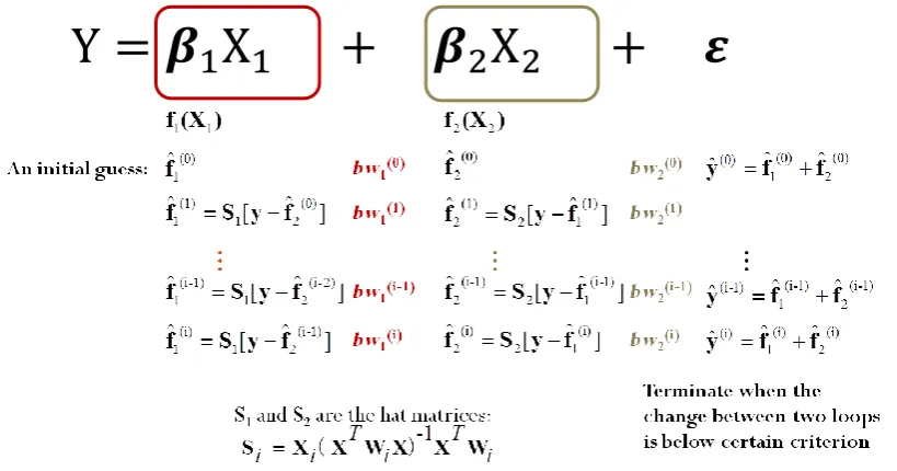
The smooth functions can be estimated by a local scoring algorithm (Hastie and Tibshirani, 1986), with the additive model estimated by an iterative procedure of back-fitting (Mosteller and Tukey, 1977, Friedman and Stuetzle, 1981, Breiman and Friedman, 1985). The back-fitting method will be demonstrated in more detail in Chapter 4.

GAM can be seen as a data-driven model, where the nature of the relationships between the dependent variable and independent variables is suggested by the data, rather than being prespecified by a given parametric form (Yee and Mitchell, 1991). It provides more flexibility than the linear parametric model and has been widely used in modelling complex nonlinear relationships. Applications can be seen in economics (Deaton and Muellbauer, 1980), ecology (Guisan et al., 2002), environmental sciences (Wood and Augustin, 2002) and many other areas.

However, because of its flexibily, caution needs to be exercised when applying GAM in order not to over-fit the data (Hastie and Tibshirani, 1990). In addition, although the additive structure of GAM provides more interpretability than a general high dimensional regression surface (Buja et al., 1989), allowing the effect of each independent variable on the dependent variable to be examined seperately, GAM is not as easily interpreted as a linear model and the results of GAM are not easily summarized and communicated (Hastie and Tibshirani, 1986).

15

The above developments in non-spatial regression models can be employed in spatial regression but the spatial effects of spatial autocorrelation and spatial non-stationary which usually violate the assumptions of non-spatial regression models are not explicitly incorporated and new techniques are thus required to be developed for the use of spatial data. These are now introduced.

2.4 Spatial regression models

Spatial regression models refer to models that have been developed from traditional regression to make them applicable to spatial data, taking spatial autocorrelation and spatial non-stationarity into account. Methods of spatial regression were initially applied at the global levels; the results of the models being therefore constant across the study region forming a global statement of the spatial processes under study. The realization of spatial non-stationarity in relationships between explanatory variables and a response variable in a regression model has lead to the development of local methods of spatial regression that allow for spatially varying coefficients. Instead of assuming global statements, local methods of spatial regression focus on identifying spatial variations in spatial process; the results being local estimates of regression parameters. This section gives a brief review of both global methods and local methods of spatial regression.

2.4.1

Global methods

Two traditional spatial regression models are the spatial autoregressive model and the spatial error model (Ord, 1975, Anselin, 1988), which are both global methods.

The spatial autoregressive model (SAR) (Ord, 1975, Anselin, 1988), also referred to as a spatial lagged model, is one of the most commonly used spatial process specifications to account for spatial effects. The original form of SAR is:

Y , (2-6)

16

The weighting matrix measures the spatial dependence between all pairs of observations associated with different spatial units, based on spatial contiguity, distance or other specifications of proximity. Suppose there are spatial units, will be an matrix with zero on the diagonal suggesting that a spatial unit cannot be related to itself. The auroregressive parameter is an overal measurement of spatial dependency. The model can be calibrated using maximum likelihood (Anselin, 1988) or the generalized method of moments (Kelejian and Prucha, 1998).

SAR produces a global model because it relates all spatial units in the system to each other, although for small values of the covariance between observations associated with two spatial units may approach zero when the distance between the units is larger than a certain value.

SAR is a basic framework for spatial regression and it can be expanded to various forms. The autoregressive parameter can not only be defined on the dependent variable as in equation (2-6), but can also be defined on independent variables, the error term, or a combination of these terms. When it is present in the error term, the model turns into the so-called spatial error model (SEM). All these models have been widely applied. Various extensions have been developed on the SAR framework, for example, the biparametric model (Brandsma and Ketellapper, 1979), spatial Durbin model (Burridge, 1981) and SAR with various forms of weighting matrix (Hepple, 1995, Bavaud, 1998, Getis and Aldstadt, 2004, Aldstadt and Getis, 2006).

17

2.4.2

Local methods

The purpose of local regression models is to investigate the spatial heterogeneity in model behaviour and therefore to suggest a more accurate model specification. Several such regression models are introduced in the following sub-sections.

Spatial expansion model

The spatial expansion model serves as one of the initial treatments of spatial heterogeneity and is a special case of the expansion model (Casetti, 1972) which was initially designed as a method for the construction and modification of models. The expansion model starts from an initial model where the estimates of the parameters exhibit some instability over the study area. The expansion method then relates the parameters to some new variables, makes the parameters functions of them, and generates a new model which can remove the instability in the parameter estimates so as to increase predictability or to test specific theoretical hypotheses.

Assume an initial model describing a linear relationship between a dependent variable and independent variables :

(2-7)

where are the parameters to be estimated, is the random error.

If the parameters vary over space, it is possible that their values might be related to other contextual variables across the space. The model may be expanded by assuming each parameter to be a function of contextual variables which can be chosen according to existing information or theoretical considerations about the real world phenomena. A variety of terminal models may be constructed depending on which contextual variables are chosen and what functional relationships are proposed. Particularly, the parameters can be assumed as functions of location. For example, linear expansion functions can be defined as following:

…

(2-8)

18

(2-9)

can be estimated by ordinary least squares and then

compose parameter estimates for , which are spatially varying. The

testing of the expansion model can be carried out by testing the null hypotheses that parameters are not significantly different from zero.

More complex, non-linear expansion functions can also be defined, although this will increase the complication in the estimation of the parameters as well as in the testing of their significance. The spatial expansion model provides a systematic approach to incorporating a spatial context into a non-spatial regression model. With the spatially varying parameters, the expansion model addresses the spatial variation in parameters while preserving the structure of the initial model.

The drawback of the spatial expansion model is that it relies on pre-defined parametric forms of expansion functions to describe the trends in relationships over space rather than revealing the spatial variations in relationships directly. To enable the estimation of model, the choice of expansion functions is limited; general smooth trends are assumed in relationships and therefore the spatial variations may be simplified and some important local variations may be missed (Fotheringham and Brunsdon, 1999).

Multilevel modelling

Multilevel modelling (Aitkin and Longford, 1986, Goldstein, 1987) treats a regression model as a hierarchical system composed of regression equations at various levels. The parameters in the regression model are assumed to be random variables to be estimated from certain probability distributions which are also estimated. Consider a two-level model specification which involves a low-level model based on individual data and a high-level model based on group data. The low-level model has the form:

(2-10)

where is the dependent variable measured at individual in group , is the

independent variable measured at the same observation as , and is the random

error. The two parameters and are random variables and assumed to be

19

(2-11)

where and are the global parameters for the whole dataset, and are

randomly varying variables for group with mean zero and constant variance. Equation (2-10) can be rewritten as:

(2-12)

which is the sum of a fixed part and a random part within the brackets. As the multilevel model contains more than one residual term, traditional OLS is not applicable for parameter estimation but an iterative generalised least-squares (IGLS) algorithm can be used (Goldstein, 1986). More alternative estimation procedures are summarized by Jones (1991). The multilevel model can be extended to include more levels, more independent variables as well as nonlinear forms (Goldstein, 2010). The hierarchical structure can also be extended to a more complex underlying data structure, for example, multiple membership multiple classification model (Browne et al., 2001) has been developed so that an observation can belong to more than one member of a classification.

Multilevel modelling allows the specification of models at several different scales simultaneously and the exploration of variations between groups at the same scale. It has gained wide application in regression analysis where data have a hierarchical structure, for example, in educational data (Goldstein, 1991), longitudinal data (Orford, 2000, Huang and Clark, 2002), and other multi-scale geographical data (Jones, 1991). Among the hierarchical structures incorporated in the model, space is an important structure, i.e., the multilevel model allows relationships to vary in different spaces, making the model a useful local spatial regression model. However, the limitation of the multilevel model is that it assumes no dependence or connection between neighbouring observations or groups and the continuous nature of space is not taken into account (Fotheringham, 1997). It also requires the nature of the spatial structure to be defined a priori; a task not always possible due to lack of knowledge about what this structure might be.

Spatial filtering model

20

that the regression residuals remain uncorrelated and traditional linear regression techniques such as OLS can be applied to the filtered data.

Various spatial filtering procedures have been developed to achieve this aim. Tiefelsdorf and Griffith (2007) review the different methods from the early parametric models which aim to identify an underlying data generating spatial process (Griffith, 1979, Haining, 1991), to the more recent nonparametrical approaches based on data transformations, including the Gi-based approach developed by Getis (Getis, 1990, Getis, 1995), and the eigenvector approach by Griffith (1996).

Getis’s filtering approach is based on local autocorrelation measures, namely the local Getis Gi-statistic (Getis and Ord, 1992). The approach helps to improve the specification of multiple regression relationships but it only works on a univariate spatial pattern and therefore each variable in a regression model needs to be treated individually (Tiefelsdorf and Griffith, 2007).

Griffith’s approach is based on eigenvector decomposition using a subset of eigenvectors that are extracted from the underlying spatial structure to capture the dependencies in a regression model. This approach helps to explore the impact of spatial autocorrelation on correlation coefficients (Getis and Griffith, 2002). It can be applied to individual variables as well as to a regression system simultaneously. It can also be incorporated into generalized linear models (GLM), offering a wider range of applications. The drawback with this approach is that the calculation of eigenfunctions involves intensive computation.

Both approaches allow the use of traditional OLS for model calibration. Getis and Griffith (2002) compared the two approaches and concluded that they yield similar regression models.

Based on Griffith’s eigenvector approach, Tiefelsdorf and Griffith (2007) further developed a semiparametric eigenvector spatial filtering approach which offers more feasibility, flexibility, and simplicity. More spatial filtering methods, including another eigenvector approach based on principal coordinates of neighboring matrices (Borcard and Legendre, 2002), are reviewed by Griffith (2010).

21

Bayesian spatially varying coefficient regression

Bayesian regression models with spatially varying coefficient processes (SVC) were introduced to model non-constant linear relationships between variables in the statistics literature (Gelfand et al., 2003). In the SVC framework, the parameters are treated as unknown random quantities from a multivariate spatial process. The SVC model is constructed by adding a continuous multivariate spatial process to account for spatially varying coefficients and to accommodate spatial dependence between variables. Suppose there are observations in a geo-referenced space. A general form of SVC model is then:

̃ , (2-13)

where is the dependent variable measured for observation , is the vector of independent variables measured for and is the vector of regression coefficients which are assumed to be constant. ̃ is a sub-vector of whose regression coefficients are assumed to be spatially-varying. is the independent and identically distributed residual with zero mean and σ2 variance. follows a multivariate Gaussian process which is characterized by its mean and a

cross-covariance function. ̃ forms the vector of spatially-varying coefficients. The calibration of the model involves the choice of prior distributions for the model parameters.

The advantages of SVC are its flexibility and capacity for inference. By using complex correlation structures for the coefficient processes, SVC provides a valid probability model from which an entire posterior inference for the spatially varying coefficient processes at both observed and unobserved locations can be obtained. It enables both hypotheses tests on model parameters and uncertainty assessment on predictions.

22

Moving window regression

Moving window regression (MWR) is a straightforward local regression approach to address spatial non-stationarity in relationships between variables. It employes a similar idea to locally weighted regression lowess in non-spatial cases, that only a subset of the dataset is used to fit a separate regression model at each point. The difference is that MWR defines the subsets in a geo-referenced space rather than the attribute space as used in lowess. The procedure of MWR can be described as: each location is visited in turn in a moving window fashion, a window centered at the location is imposed and the observations situated within the window are included to conduct a regression model with local regression coefficients estimated for this location. Once all locations are visited, each location then has its own set of regression coefficient estimates which can be mapped and compared.

By calibrating various regression models for each location, MWR can capture spatial variation in processes. A key decision, however, to be made when applying MWR is the choice of the window size, which reflects the geographical scale of the spatial processes being investigated. The smaller a window size is, the more local the regression will be, while the more variance will be in the model. The effects of various window sizes and the methods to choose an optimal size have been demonstrated by applications such as Lloyd and Shuttleworth (2005) in commuting analysis and Páez et al. (2008) in house price prediction. Empirical comparison with global regression and other local regression techniques including SAR indicates that MWR produces accurate estimates and helps to identify local anomalies (Farber and Yeates, 2006).

23

Another drawback of MWR is that it is discrete (Fotheringham et al., 2002); any information contained in the observations outside of a window is totally ignored in a local regression. This may not be reasonable for a real world spatial process.

Geographically weighted regression

Moving window regression can be seen as a special case of a more sophisticated local regression framework, geographically weighted regression (GWR) (Brunsdon et al., 1996, Fotheringham et al., 1996, Brunsdon et al., 1998b, Fotheringham et al., 1998). In MWR, all observations within the window can be considered as having an equal weight of one, while all observations outside of the window have a weight of zero. GWR defines the weights in a more general way, weighting the observations at various locations according to their proximity to the centre of the window. The closer an observation is located to the centre of the window, the more weight it receives, and vice versa. This is in accordance with the geographical principle of distance decay. A weighting scheme is employed to control the distance decay. Rather than a subset of data, all data can be included in the analysis but the weighting scheme will determine which observations have non-negligible weights.

GWR explicitly takes spatial location into account and it has been considered as one of the most important developments in the treatment of spatial non-stationarity (Anselin, 2010). More details about GWR will be presented in the next chapter.

2.5 Summary

This chapter gives a brief review of spatial analysis in general and spatial regression in particular. The importance of space has been recognized in various scientific disciplines involving theoretical domains and applied domains. The two main spatial effects that spatial data bring to data analysis are spatial autocorrelation and spatial non-stationarity. To address these two affects has thus been the main task of spatial data analysis. In terms of regression, traditional non-spatial regression methods are often insufficient in analysing spatial data while various fundamental methodologies including locally weighted regression, generalized additive modelling and so on have thrown some light on the development of local spatial regression.

24

25

Chapter 3

Geographically

Weighted

Regression

3.1 Basic methodology

Geographically Weighted Regression (GWR) (Brunsdon et al., 1996, Fotheringham et al., 1996, Brunsdon et al., 1998b, Fotheringham et al., 1998) is a useful technique to model spatial dependency and spatial heterogeneity. Based on the assumption that the relationship between the observed variables varies smoothly across a geographical space, it adopts the smoothing techniques used in Locally Weighted Regression models (Cleveland, 1979, Cleveland and Devlin, 1988) in attribute space and extends them into geographical space.

In GWR, the regression is repeated at every single location, taking into account the influence of data from surrounding locations. As a result, a series of local parameters is estimated. These parameters can be mapped as a surface, representing the variation in relationships over space. In this way, GWR describes not only the relationships between variables but also any spatial non-stationarity of these relationships.

Suppose a global linear regression model has the form:

∑ (3-1)

where y_i is the response or dependent variable measured at observation point i, x_ik

) ,..., 1

(k m is the kth predictor or independent variable at observation point i, _kis

the parameter for x_ik describing the relationship between y_i and x_ik . ₀ is the

intercept and _i is the error term. When the error terms meet the condition of being

independently and identically drawn from a Normal Distribution with mean zero and

common variance 2

, the regression parameters ₀ and _{k can be estimated by}

Ordinary Least Squares (OLS), in which the value of 2 1 ˆ ( ) n i i i y y  



the n observations in the dataset, where ˆy_i stands for the predicted value.

The basic form of GWR according to Fotheringham et al. (2002) is:

0

1

( , ) ( , )

m

i i i k i i ik i

k

y  u v  u v x 



 



26

where (u_i,v_i) stands for the geographical coordinates of the i th observation.

) , (

0 ui vi

 and _k(u_i,v_i) are parameters describing the relationships around location

) ,

(u_i v_i . Other notations have the same meaning as those in the global regression

model (3-1). By allowing the parameters to be location-specific, GWR incorporates into the model any potential spatial variation in relationships.

The fundamental mechanism of GWR is that an observation point is weighted according to its proximity to the regression point (the point at which the model is locally calibrated), so that data from observations close to a regression point are weighted higher than data from observations farther away. This accords with Tobler’s first law of geography that “Everything is related to everything else, but near things

are more related than distant things” (Tobler, 1970). The weighting scheme is centred on each regression location so thateach regression point has its own weighting matrix to participate in the estimation of the locational specific parameter estimates through a Weighted Least Squaresapproach:

y

i i

i X WX) X W

T 1 T  ( ˆ  _(3-3)

where ˆ is the vector of estimated parameters at regression point _i i, X is the design

matrix which contains the values of the independent variables and a column of 1s, y

is the vector of observed values of the dependent variable.W_i is a weight matrix

conditioned on the location i with the form:

in i i i w w w w ... 0 0 0 . ... . . . 0 ... 0 0 ... 0 0 0 ... 0 0 3 2 1  i W (3-4) This is an n by n square matrix with all the off-diagonal elements zero and the diagonal elements ranging from zero to one representing the weights of observation

points from 1 to n for the regression point i, e.g. w_i1 stands for the weight of data

from observation point 1, w_i2 is the weight of data from observation point 2, and so

27

The weighting matrices are obtained through a function of distance W(d), named a weighting function or a kernel. The general requirements for a weighting function as stated by Brunsdon et al. (1998) are:

(1) a monotone decreasing function for positive real numbers, to guarantee that the weight decreases as the distance increases;

(2) W(0) = 1, so that the observed data at the regression point contributes fully to the regression;

(3) , so that data from infinite distances hardly contribute to the

regression.

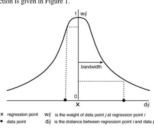
A typical function is given in Figure 1.

(Fotheringham et al., 2002, P.44)

Figure 3-1 A typical weighting function

where  marks the regression point and the curve describes how the weight varies from one to close to zero according to the distance between the data point and the regression point. If a data point is far from , the weight will be small, while if a data point is close to , the weight will be large. If the data point is at the same location as the regression point, the weight will be the maximum value of one. It is worth noticing that the distance here is a general measurement of the proximity between spatial locations and it can be measured either in Euclidean distance or in some other meaningful type of distance according to the nature of the application.

28 2 ) ( 2 1 h d ij ij e

w  

(3-5)

where w_ij is the weight of the observation point i for the regression point j, d_ij is

the distance between point iand point j, h is known as a bandwidth and determines

the size of the kernel and controls the rate of distance-decay in the weighting mechanism. The larger h _{is, the slower the weight will decay with} dij. When h

tends to infinity, the weight will tend to 1 for all values of d_ij; in this case, the model

is approximate to a global regression model. Another useful kernel is the bi-square function:

2 2 [1 ( ij) ]

ij

d w

h

  if d_ij h

0

 _{otherwise (3-6)}

The difference between this kernel and a Gaussian kernel is that the bi-square excludes those observations beyond an influence distance of h by setting their weights to zero. This property reduces the computational cost of weights, making the model computationally more efficient; moreover, this property is in accordance with our understanding of many spatial processes.

The Gaussian and bi-square are the two most frequently used kernels although there are many other kernel functions that could be utilised depending on the spatial process being studied such as, for example, the tri-cube kernel function used by McMillen and McDonald (2004). A kernel function is usually conditioned by a general constant, the bandwidth. The bandwidth determines the rate at which the weights decay. A large bandwidth allows the weights to decrease slowly while a small bandwidth allows the weights to decay quickly.

29

area and the parameter estimates will depend on observations in close proximity to the regression point. Therefore the variance of the parameter estimates will increase but the bias in them will be small and more anomalies can be discovered.

Several data-driven approaches have been developed to select an optimal bandwidth for a given dataset, such as using cross-validation (CV) to minimize prediction error and using Akaike Information Criterion (AIC) to balance between goodness of fit and complexity of the model (Fotheringham et al. 2002). Whichever criterion is used, however, the result will be a constant optimal bandwidth for the model, all the relationships in the model will then be examined based on this bandwidth.

From the perspective of weighting, a global regression model can be considered as a special case of GWR where the weights are constant and equal to one for all regression points over all the dataset. Equally, moving window regression can be seen as having a boxcar function as the kernel:

if ℎ

otherwise (3-7)

where the bandwidth h equal to the window size. In this sense, GWR can be viewed as a general framework for a variety of regression models.

Although GWR was first introduced as an exploration tool to detect spatial non-stationarity in relationships between variables, the GWR estimates in the form of 3-3 provide a reasonable fit to the model in 3-2. It has been shown that, with the assumptions of independently normally distributed error terms having mean zero and

common variances in formula (3-2), the least squares estimates of _k(u_i,v_i) are

equivalent to estimates from a maximum likelihood approach (Fotheringham et al., 2002). Therefore GWR can be a statistical model with proper statistical inferences. Classical inference techniques, such as significance tests, confidence intervals, model comparison also apply to GWR.

3.2 Use of GWR

Since its introduction, GWR has proven to be a popular tool for the study of geo-referenced data and has been applied widely from social to natural sciences. The purpose of using GWR includes exploration, visualisation and prediction.

30

et al., 1996). Fotheringham et al. (1998) suggested using it as a diagnostic to improve spatial understanding. Since the main outputs of GWR are the spatial variations in parameter estimates, these spatial variations can help to uncover interesting patterns in relationships, raise new research questions and guide further investigation into the processes being studied. Applications of GWR as an exploratory tool can been found in diverse disciplines, such as, ecology and environment (Foody, 2003, Pavel et al., 2008, Kupfer and Farris, 2007), climatology (Brunsdon et al., 2001), urban poverty (Longley and Tobón, 2004), regional science (Farber and Yeates, 2006, Huang and Leung, 2002), health and disease analysis (Nakaya et al., 2005b), environmental justice (Mennis and Jordan, 2005) and political science (Darmofal, 2008, Cho and Gimpel, 2010).

31

approaches in producing accurate spatial predictions. For example, Gao et al. (2006) evaluate the prediction power of GWR together with a global linear regression model, a spatial dependency model, and a GWR mixed with spatial dependency model, through a house and land price dataset. Results show the superior performance of GWR on several empirical criteria. Kupfer and Farris (2007) apply GWR to predictive vegetation modelling and conclude that the prediction results from GWR had a closer fit to observed values with lower residuals than those from a global linear regression model. Bitter et al. (2007) compare GWR and the spatial expansion model in examining spatial heterogeneity in housing attribute prices within Tucson, Arizona and conclude that GWR outperforms the spatial expansion model in terms of explanatory power and predictive accuracy and that when explanatory power and predictive accuracy are the primary objectives of study, GWR is the superior approach. Lloyd (2010b) illustrates the benefits of local approaches including MWR and GWR against global regression for the characterization of spatial variation and for prediction. Simple kriging with local means (SKlm) conducted using local variograms estimated from GWR is also demonstrated. Harris et al. (2010b) compared GWR as a predictor with global multiple linear regression (MLR) and traditional geostatistical models of kriging, as well as a GWR based kriging (GWRK) where kriging models are specified with GWR as a mean component. Tests on simulated data with different levels of spatial heterogeneity and spatial autocorrelation show that both GWR and GWRK predictors performed better than MLR and ordinary kridging and that they could act as alternatives to the usually preferred kriging with external drift (KED) when predicting with non-stationary relationships.