Groundwater Solution Techniques: Environmental Applications

Groundwater Solution Techniques: Environmental

Applications

Sarva Mangala PRAVEENA1*_{, Mohd Harun ABDULLAH}1_{, Ahmad Zaharin ARIS}2_{, Kawi BIDIN}1

1_{School of Science and Technology, Universiti Malaysia Sabah, Kota Kinabalu, Sabah, Malaysia.} 2_{Department of Environmental Sciences, Universiti Putra Malaysia, Selangor, Malaysia}

E-mail: [email protected]

Received September 29, 2009; revised October 29, 2009; accepted November 14, 2009

Abstract

Groundwater models provide a scientific tool for various groundwater studies which include groundwater flow, solute transport, heat transport and deformation. However, without a good understanding of a model, modeling studies are not well designed or the model does not represent the natural system which being mod-eled long term effects may results. Thus, this review has focused and reviewed the types of solution tech-niques in terms of advantages and limitations. The findings are vital to improve the model conceptualization and understanding of the uncertainty in model results. On the same hand, it acts as guide and reference to groundwater modeler, reduces the time spent in understanding the solution technique and complexity of groundwater models, as well as focus ways to address the groundwater problems and deliver modeling out-put more efficiently.

Keywords: Groundwater Models, Solution Techniques, Advantages, Limitations

1. Introduction

According to [1], groundwater modeling covers dif-ferent aspects of the system behavior. Groundwater modeling studies have four potential relevance proc-esses which include groundwater flow, solute transport, heat transport and deformation. According [2,3], groundwater modeling has turn out to be a crucial tool in decision making and planning in environmental management. Decision making and planning processes in environmental management are associated with wa-ter resource allocation, complex development and re-quiring multidisciplinary information for evaluating their effects on a social, economic and environmental level [4]. Generally, most of the groundwater modeling studies are conducted using either deterministic models, based on precise description of cause-and-effect or stochastic models based on the probabilistic nature of a groundwater system [5,6]. The main components of groundwater modeling are selecting the natural sys-tem which the model is designed, creating the concep-tual representing the natural system, models represent-ing the controllrepresent-ing mechanism, solution of the model, calibration and validation of the model along with simulation [7,8].

There are enormous amount of groundwater models

to study the cause and effect or the probabilistic nature of a groundwater system. It is an ad-vantage to classify them in groups based on criterias such as aquifer type, techniques used, type of aquifer simulated and the di-mension of the problem [9]. [10] stated that the classi-fication of groundwater models can be done based on model objectives, processed modeled, physical system characteristics modeled and mathematical approaches. According to International Ground Water Modeling Center (IGWMC), there are many various manners in groundwater models classifications (flow, media, trans- port, temperature, phases, chemical reaction, disper-sion, thermodynamics, fractured rock, vapor transport, variable saturated, saturated) that a specific and sys-tematic classification cannot be developed. A detailed explanation of these classifications can be found in [10].

universal importance perspective. Era of numerous groundwater models development has been stimulated by high advance of computer technology and pro-gramming techniques. Yet the current numerous model development and groundwater complexity often leave those involve in groundwater studies spend a lot of time in understanding the solution techniques. This increased time resulted in less time spent in under-standing the system. Thus, there are many gaps in our understanding of groundwater modeling which limits our capacity. Various groundwater models develop-ment have exposed with many reviews on the favors and disfavors of these models [6,8,11]. However, there are limited reviews on the solution techniques of these groundwater models although they are crucial compo-nents utilized in groundwater modeling. While a num-ber of these solution techniques are focused on the types of models and applications in real world [11–14], a lack of quantitative information on the advantages and limitations of these tools impedes the use of these tools for real-world applications.

An understanding of various solution techniques is crucial due to complexity in groundwater modeling. This work was intended primarily as a guide and ref-erence for the practitioner who is trying to simulate groundwater in their site of interest. This attempt is a way to lessen the time spent in understanding the solu-tion technique and complexity of groundwater models, as well as focus ways to address the groundwater problems to render modeling output more effectively. The conceptual framework of the review was based on the types of solution techniques available in ground-water studies. An assessment of mutual understanding, advantages and limitations of all the solution tech-niques is applied to all kind of groundwater modeling studies and not limited to any particular purpose or equations. It is an attempt to reduce the time spent in understanding the solution technique and complexity of groundwater models and represent focus ways to address the groundwater problems and render modeling output more effectively.

2. Various Solution Techniques Assessment

According to [8], the term model has different meanings. Combinations of all model components are suitable for groundwater model. However, term model is also used in a part of various solution techniques. Thus, the term model will also be used in a part of solution technique in this review. Numerous sophisticated solution techniques or model are currently available to overweigh the accu-racy of the groundwater system representation [15]. The groundwater solution techniques comprise from simple to complex [6]. According to [2] until early 1970s, physical and analog models were widely used as

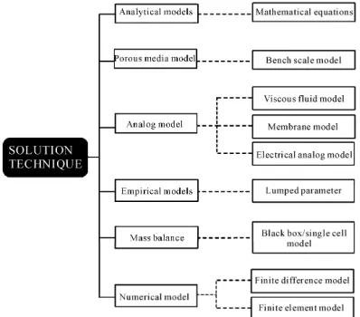
mathe-matical models solving groundwater problems. As groundwater modeling techniques boosted with extensive computer programmings, various solution techniques have been developed to solve the systems of mathemati-cal equations. The simplest classification was done by [12] and [14], where the solution techniques are divided into two broad groups namely physical models and mathematical or numerical models. Solution techniques grouping done by [11] listed that groundwater models are divided into four broad groups which are porous me-dia, analog, electric analog and digital models. Along with the advent of computers, groundwater modeling has focused on the numerical models expressing the ground- water flow and transport studies. However, these models (analytical, physical, analog, porous, empirical and mass balance) are still needed to investigate and validate new models. The requirements are to examine and analyze whether certain assumptions underlie the new models are valid. The conceptual framework of this review was based on the types of solution techniques listed by [8] as showed in Figure 1.

3.

Solution Techniques Evaluations

It is very important to have strong understanding with a model in order to know the advantages and limitations of each solution techniques. Perspectives of advantages and limitations of the solution techniques were evaluated in this review.

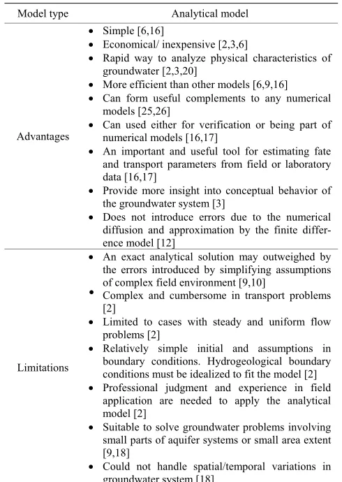
3.1. Analytical Models

Analytical models are the rapid way to analyze physical characteristics and conceptual behavior of groundwater system compare to other models. This is because it uses an exact analytical solution for specific field applications. On the other hand, analytical models are only limited to steady and uniform groundwater problems involving

small parts of study area and bulky to transport problems. Table 1 presents other points of advantages and limita-tions of analytical models.

3.2. Porous Media Models

Porous media or bench-scale models belong to the group of hydraulic models which has been widely used in hy-draulic engineering. Porous media models are suitable to use at any dimensionality, any type of groundwater flow and transport problems (variable saturated, heterogeneity, anisotropy, phreatic, steady, unsteady, advection, disper-sion, sorption, decay and reactions). Information about porous media is presented in Table 2.

3.3. Analog Models

In terms of demonstration and education tools, analog models are still widely used for groundwater studies. Analog models (viscous fluid, membrane and lumped models) are not suitable for groundwater transport. The models have limited capability to involve with advection, dispersion, sorption, decay and reactions studies in

Table 1. Applicability of analytical models.

Model type Analytical model

Advantages

 Simple [6,16]

 Economical/ inexpensive [2,3,6]

 Rapid way to analyze physical characteristics of groundwater [2,3,20]

 More efficient than other models [6,9,16]

 Can form useful complements to any numerical models [25,26]

 Can used either for verification or being part of numerical models [16,17]

 An important and useful tool for estimating fate and transport parameters from field or laboratory data [16,17]

 Provide more insight into conceptual behavior of the groundwater system [3]

 Does not introduce errors due to the numerical diffusion and approximation by the finite differ-ence model [12]

Limitations

 An exact analytical solution may outweighed by the errors introduced by simplifying assumptions of complex field environment [9,10]

 _{Complex and cumbersome in transport problems}

[2]

 Limited to cases with steady and uniform flow problems [2]

 Relatively simple initial and assumptions in boundary conditions. Hydrogeological boundary conditions must be idealized to fit the model [2]

 Professional judgment and experience in field application are needed to apply the analytical model [2]

 Suitable to solve groundwater problems involving small parts of aquifer systems or small area extent [9,18]

 Could not handle spatial/temporal variations in groundwater system [18]

groundwater. The views on advantages and disadvan-tages of analog models are detailed in Table 3.

3.4. Empirical Models

Empirical models are useful to use when detailed site specific data are lacking or impractical situation to simu-late fine-scale processes. Lack of understanding in the

Table 2. Applicability of porous media models.

Model type Porous media model

Advantages

 _{Relatively straightforward and simple [19,}

20]

 Allow the study of special aspects of groundwater flow and transport under al-most natural condition [19,20]

 Useful to enhance site characterization and features [9]

 _{Good demonstration and education tools for}

students [4,7,20]

 Obeys laws that govern other physical systems including laminar flow of fluids and heat [4,6,7]

 Good starting point for groundwater mod-eling beginners [4]

Limitations

 Capillary rise takes place in such models is far larger than that which actually occurs in a real field situation [13]

 Difficult to visual and identify the water table [7,13]

 Time consuming and prohibitively costly [5]

Table 3. Applicability of analog models.

Model type Analog model

Advantages

 Illustrative and still widely used for demon-stration purposes of groundwater flow [4,21]

 Versatility and can readily study a variety of aquifer conditions [8]

 True for groundwater flow without natural recharge if the weight of the membrane is small [4]

 Inexpensive tools to use to visualize groundwater stress [4]

 Useful tool to help the inexperienced earth scientist to understand about groundwater hydraulics [4]

 Solves problems concerning the phreatic surface for transient and steady flow con-ditions[4,7,21]

Limitations

 _{A good care is required in the model}

con-struction because flow rate varies with the cube width [4,7]

 _{Temperature is also another factor need to}

be focused [4,5]

 _{Limitation on applications involving}

nonlinear conditions of varying transmis-sivity in unconfined aquifers and two-fluid flow problems [7,13]

 _{Also limited applications in groundwater}

lowering in construction field [21]

 _{Electric potential is unaffected by gravity,}

processes involve in study area, these models can be misused or misunderstood as the models are easy to em-ploy as well as lumping process together will mask the disadvantages of these models. Table 4 summarizes the information on empirical models.

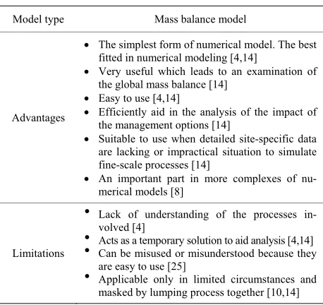
3.5. Mass Balance Models

Mass balance model is also known as the black box or single-cell model. It is also a numerical model in its sim-plest form. In mass balance models, the averaging of an entire area is a crude approximation. Evaluation of field data is only involves in and out fluxes. Table 5 details the information of mass balance models.

Table 4. Applicability of empirical model.

Model type Empirical model

Advantages

 Impact the accuracy of the model predictions [23,24]

 Suitable to use when detailed site specific data are lacking and appropriate when it is imprac-tical to simulate fine-scale processes [4]

 Representing an entire groundwater problem employs a series of physical laws, empirical laws and conservative assumptions to represent the problem of interest [1,4,23,24]

 A good alternative method [23,24]

 Provide useful predictions without the costly calibration time [23,24]

Limitations

 _{Lack of understanding of process involved and}

only a temporary solution to assist analysis [7, 24]

 Can be misused and misunderstood because they are easy to employ [4]

 Lumping processes together will mask the limitations of these models [7]

Table 5. Applicability of mass balance model.

Model type Mass balance model

Advantages

 The simplest form of numerical model. The best fitted in numerical modeling [4,14]

 Very useful which leads to an examination of the global mass balance [14]

 Easy to use [4,14]

 Efficiently aid in the analysis of the impact of the management options [14]

 Suitable to use when detailed site-specific data are lacking or impractical situation to simulate fine-scale processes [14]

 An important part in more complexes of nu-merical models [8]

Limitations

 _{Lack of understanding of the processes}

in-volved [4]

 _{Acts as a temporary solution to aid analysis [4,14]}  _{Can be misused or misunderstood because they}

are easy to use [25]

 _{Applicable only in limited circumstances and}

masked by lumping process together [10,14]

3.6. Numerical Models

Among of the solution techniques assessment, numerical models were found to have more advantages over other solution techniques. They are such as it solves both sim-ple and comsim-plex groundwater problems, capable to used almost of any type of groundwater system and impose no restrictions on the initial conditions, boundary types as well as characteristics of the groundwater. The most ad-vantage in numerical models is that the models utilize the latest advances in computer technology without writing any computer codes. Numerical models which employ the latest computer technology also have limitations in terms of accuracy, errors and codes. Accuracy of nu-merical output mainly depends on the availability of soil hydraulic information, errors in numerical dispersion are hard to be identified as well as special codes are need for specific groundwater problem (Table 6).

Table 6. Applicability of numerical model.

Model type Numerical model

Advantages

 _{Employed with the latest and recent advances in}

computer technology [4,5,11,13]

 Solves both simple and complex groundwater problems [4,7,13,26,27]

 Dominated the complex study of groundwater problems as it solves both simple and complex one, two or three dimensional problems [4,7,13, 15]

 Capable to simulate almost any type of ground-water situation [5,7,17]

 Well suited to exploring hypothetical scenarios [15,27]

 _{Can easily handle spatial or temporal variations}

of groundwater system [6,11]

 _{Impose no restrictions on the initial conditions,}

boundary types, characteristics of the ground-water or investigated solute [5,10]

 Computer programs for most groundwater

problems are available easily and the users can apply relevant computer programs without writ-ing any computer code [4,7,13,26,27]

Limitations

 _{Time consuming for data collection and input}

[4,7,11,13]

 Require much information to characterize the system [28]

 Expensive models [28]

 Special codes are required for specific problems, such as density-dependent flow and coupled saturated unsaturated flow [15,27]

 Accuracy of the results of numerical models mainly depends on the availability of informa-tion about the hydraulic properties of the subsoil [28]

 Errors in numerical dispersion [28]

4. Conclusions

This review has focused and reviewed the types of solu-tion techniques available in groundwater modeling stud-ies. Assessment of six solution techniques namely ana-lytical, porous media, analog, empirical, mass balance and numerical models was done to give a clear under-standing of each solution techniques. Advantages and limitations of all the solution techniques were listed and analyzed. Analytical, porous media and mass balance models are simple and appropriate to use in groundwater modeling studies. In terms of demonstration and educa-tion tools, porous media and analog models are still widely used for groundwater studies. Empirical and mass balance models are useful to use when detailed site spe-cific data are lacking or impractical situation to simulate fine-scale processes. The most benefit of numerical models is it utilizes the latest advances in computer technology without writing any computer codes as well as solves both simple and complex of any groundwater problems. On the other hand, limitations of analytical models are only limited to steady and uniform ground-water problem involving small parts of study area. Po-rous media and numerical models face time consuming for data collection and expensive as their constraints in the applications. Empirical and mass balance models face lack of understanding in the processes involve in study area and can be misused or misunderstood. In the view of analog models, they are not suitable for ground-water transport. Moreover, errors in numerical dispersion are hard to be identified as well as special codes are need for specific groundwater problems. As a final note, it is important to point out that a good understanding of vari-ous solution techniques act as guide and reference to groundwater modeler. Besides, it reduces the time spent in understanding the solution technique and complexity of groundwater models, as well as focus ways to address the groundwater problems and render modeling output more effectively.

5. Acknowledgement

The first author gratefully acknowledges the support by National Science Fellowship (NSF) Scholarship under sponsorship of Ministry of Science, Technology and In-novation (MOSTI), Malaysia for her doctoral study. Sincere appreciation is also extended to the reviewers for their helpful comments and suggestions which have im-proved the quality of this paper.

6. References

[1] L. W. Canter, D. M. Fairchild, and R. C. Knox, “Ground water quality protection,” CRC Press, Boca Raton,

Flor-ida, 1988.

[2] J. Bear, M. S. Beljin, and R. R. Ross, “Fundamentals of groundwater modeling,” United States Environmental Protection Agency, 1992.

[3] P. K. M. van der Heijde, “Quality assurance in computer simulations of groundwater contamination,” Environ-mental Software, Vol. 2, pp. 19–25, 1987.

[4] E. Manoli, P. Katsiardi, G. Arampatzis, and D. Assima-copoulos, “Comprehensive Water Management Scenarios for Strategic Planning,” Global NEST Journal, Vol. 7, pp. 369–378, 2005.

[5] S. M. Praveena, M. H. Abdullah, A. Z. Aris, and L.C. Yik, “A brush up on seawater intrusion models,” in the Pro-ceeding of Third Regional Symposium on Environment and Natural Resources, Kuala Lumpur, pp. 313–324, 2008.

[6] C. P. Kumar, “Pitfalls and sensitivities in groundwater modeling,” Civil Engineering, Vol. 84, pp. 116–120, 2003. [7] V. S. Singh and C. P. Gupta, “Groundwater in a coral is-land,” Environmental Geology, Vol. 37, pp. 72–77, 1999. [8] K. Spitz and J. Moreno, “A practical guide to

groundwa-ter and solute transport modeling,” John Wiley and Sons, New York, 1996.

[9] M. E. Thangarajan, “Resource evaluation, augmentation, contamination, restoration, modeling and management,” Capital Publishing Company, 2007.

[10] J. R. Boulding and J. S. Ginn, “Practical handbook of soil, vadose zone, and ground-water contamination: Assess-ment, prevention and remediation,” Lewis Publishers, Boca Raton, Florida, 2004.

[11] D. K. Todd, “Groundwater hydrology,” Second Edition. John Wiley & Sons, New York, 1980.

[12] M. P. Anderson and W. W. Woessner, “Applied ground-water modeling: Simulation of flow and advective trans-port,” Academic Press, Inc., San Diego, 2002.

[13] N. Krešić, “Hydrogeology and groundwater modeling,” CRC Press, Boca Raton, Florida, 2006.

[14] W. C. Walton, “Groundwater resource evaluation,” McGraw-Hill Education, 1976.

[15] K. McGillicuddy and T. Sovich, “Strategies for operation of orange county water district Talbert seawater intrusion barrier, California,” ASCE, New York, 1996.

[16] A. M. M. Elfeki, G. J. M. Uffink, and F. B. J. Barends, “Groundwater contaminant transport: Impact of hetero-geneous characterization: A new view on dispersion,” Taylor & Francis, 1997.

[17] N. Emekli, N. Karahanoglu, H. Yazicigil, and V. Doy-uran. “Numerical simulation of saltwater intrusion in a groundwater Basin,” Water Environment Research, Vol. 68, pp. 855–866, 1996.

[18] L. F. Konikow and T. E. Reilly, “Groundwater model-ing,” In: The Handbook of Groundwater Engineering, CRC Press, Boca Raton, Florida, 1995.

379–409, 1988.

[20] J. J. Fried, “Groundwater pollution: Theory, methodology, modelling, and practical rules,” Elsevier Scientific Pub-lishing Company; Amsterdam-Oxford-New York, 1975. [21] R. Bowen, “Groundwater,” Springer; London, 1986. [22] J. Wainwright and M. Mulligan, “Environmental

model-ing: finding simplicity in complexity,” John Wiley and Sons, New York, 2004.

[23] K. R. Rushton, “Groundwater hydrology: Conceptual and computational models,” John Wiley & Sons, New York, 2003.

[24] Environmental Protection Agency, “Models and com-puters in ground-water investigations,” 1991, http://www.

cepis.ops-oms.org/muwww/fulltext/repind46/models/mod els.html.

[25] V. Batu, “Applied flow and solute transport modeling in aquifers: fundamental principles and analytical and nu-merical methods,” CRC Press, Boca Raton, Florida, 2006. [26] G. B. Maxey, W. Back, and D. A. Stephenson

“Contem-porary hydrogeology,” The George Burke Maxey memo-rial volume, Elsevier, 1979.

[27] M. Kasenow, “Determination of hydraulic conductivity from grain size analysis,” Water Resources Publication, 2002.