FIRST ASSESSMENT OF THE BINARY LENS OGLE-2015-BLG-0232.
E. BacheletR0, V. BozzaS0,S1, C. HanC0, A. UdalskiO0, I.A. BondM0, J.-P. BeaulieuP0,P1, R.A. StreetR0, J.-I KimC1 and,
D. M. BramichR1, A. CassanR2, M. DominikR3,†, R. FigueraJaimesR7,R3,R4, K. HorneR3, M. HundertmarkR5,R6, S. MaoR7,R8,R9J. MenziesR10, C. RancR2, R. SchmidtR6, C. SnodgrassR11, I. A. SteeleR12, Y. TsaprasR6, J. WambsganssR6,
(TheRoboNet collaboration)
P. Mroz´ O0, I. Soszynski´ O0, M.K. Szymanski´ O0, J. SkowronO0, P. PietrukowiczO0, S. KozłowskiO0, R. PoleskiO1, K. UlaczykO0, M. PawlakO0, (TheOGLEcollaboration)
F. AbeM2R. BarryM3D. P. BennettM3,M10A. BhattacharyaM3,M10M. DonachieM4A. FukuiM5,M13Y. HiraoM1Y. ItowM2K. KawasakiM1I. KondoM1N. KoshimotoM11,M12M. CheungAlexLiM4Y. MatsubaraM2Y. MurakiM2S. MiyazakiM1M. NagakaneM1N. J. RattenburyM4H.
SuematsuM1D. J. SullivanM6T. SumiM1D. SuzukiM9P. J. TristramM7A. YoneharaM8 (TheMOAcollaboration)
R0Las Cumbres Observatory, 6740 Cortona Drive, Suite 102, Goleta, CA 93117 USA
R1New York University Abu Dhabi, PO Box 129188, Saadiyat Island, Abu Dhabi, UAE
R2Sorbonne Universit´es, UPMC Univ Paris 6 et CNRS, UMR 7095, Institut d’Astrophysique de Paris, 98 bis bd Arago, 75014 Paris, France
R3SUPA, School of Physics & Astronomy, University of St Andrews, North Haugh, St Andrews KY16 9SS, UK
R4European Southern Observatory, Karl-Schwarzschild-Str. 2, 85748 Garching bei M¨unchen, Germany
R5Niels Bohr Institute & Centre for Star and Planet Formation, University of Copenhagen, Øster Voldgade 5, 1350 - Copenhagen K, Denmark
R6Zentrum f¨ur Astronomie der Universit¨at Heidelberg, Astronomisches Rechen-Institut, M¨onchhofstr. 12-14, 69120 Heidelberg, Germany
R7Pysics Departement and Tsinghua Centre for Astrophysics, Tsinghua University, Beijing 100084, China
R8National Astronomical Observatories, Chinese Academy of Sciences, 20A Datun Road, Chaoyang District, Beijing 100012, China
R8Jodrell Bank Centre for Astrophysics, School of Physics and Astronomy, The University of Manchester, Oxford Road, Manchester M13 9PL, UK
R9South African Astronomical Observatory, PO Box 9, Observatory 7935, South Africa
R10Planetary and Space Sciences, Department of Physical Sciences, The Open University, Milton Keynes, MK7 6AA, UK
R11Astrophysics Research Institute, Liverpool John Moores University, Liverpool CH41 1LD, UK
C0Department of Physics, Chungbuk National University, Cheongju 28644, Korea
C1Korea Astronomy and Space Science Institute, Daejon 34055, Korea
O0Warsaw University Observatory, Al. Ujazdowskie 4, 00-478 Warszawa,Poland
O1Department of Astronomy, Ohio State University, 140 W. 18th Ave.,Columbus, OH 43210, USA
M0Institute of Natural and Mathematical Sciences, Massey University, Auckland 0745, New Zealand
M1Department of Earth and Space Science, Graduate School of Science, Osaka University, Toyonaka, Osaka 560-0043, Japan
M2Institute for Space-Earth Environmental Research, Nagoya University, Nagoya 464-8601, Japan
M3Code 667, NASA Goddard Space Flight Center, Greenbelt, MD 20771, USA
M4Department of Physics, University of Auckland, Private Bag 92019, Auckland, New Zealand
M5Subaru Telescope Okayama Branch Office, National Astronomical Observatory of Japan, NINS, 3037-5 Honjo, Kamogata, Asakuchi, Okayama 719-0232,
Japan
M6School of Chemical and Physical Sciences, Victoria University, Wellington, New Zealand
M7University of Canterbury Mt. John Observatory, P.O. Box 56, Lake Tekapo 8770, New Zealand
M8Department of Physics, Faculty of Science, Kyoto Sangyo University, 603-8555 Kyoto, Japan
M9Institute of Space and Astronautical Science, Japan Aerospace Exploration Agency, 3-1-1 Yoshinodai, Chuo, Sagamihara, Kanagawa, 252-5210, Japan
M10Department of Astronomy, University of Maryland, College Park, MD 20742, USA
M11Department of Astronomy, Graduate School of Science, The University of Tokyo, 7-3-1 Hongo, Bunkyo-ku, Tokyo 113-0033, Japan
M12National Astronomical Observatory of Japan, 2-21-1 Osawa, Mitaka, Tokyo 181-8588, Japan
M13Instituto de Astrof´ısica de Canarias, V´ıa L´actea s/n, E-38205 La Laguna, Tenerife, Spain
S0Dipartimento di Fisica ”E.R. Caianiello”, Universit`a di Salerno, Via Giovanni Paolo II 132, 84084, Fisciano, Italy
S1Istituto Internazionale per gli Alti Studi Scientifici (IIASS), Via G. Pellegrino 19, 84019 Vietri sul Mare (SA), Italy
P0 School of Physical Sciences, University of Tasmania, Private Bag 37 Hobart, Tasmania 7001 Australia; [email protected]
P1 Sorbonne Universit´es, UPMC Universit´e Paris 6 et CNRS, UMR 7095, Institut d’Astrophysique de Paris, 98http://www.plt.axvline/bis bd Arago, 75014
Paris, France; [email protected] and †Royal Society University Research Fellow
(Received receipt date; Revised revision date; Accepted acceptance date)
Draft version November 8, 2018
ABSTRACT
We present an analysis of the microlensing event OGLE-2015-BLG-0232. This event is challenging to charac-terize for two reasons. First, the light curve is not well sampled during the caustic crossing due to the proximity of the full Moon impacting the photometry quality. Moreover, the source brightness is difficult to estimate because this event is blended with a nearby K dwarf star. We found that the light curve deviations are likely due to a close brown dwarf companion (i.e., s =0.55 andq = 0.06), but the exact nature of the lens is still unknown. We finally discuss the potential of follow-up observations to estimate the lens mass and distance in the future.
Keywords:gravitational microlensing
1. INTRODUCTION Twenty years after the first exoplanet detection, it is clear that planets are abundant in the Milky Way (Cassan et al.
2012; Fressin et al. 2013; Bonfils et al. 2013; Clanton & Gaudi 2016; Suzuki et al. 2016). But the dividing line between super-Jupiter and brown dwarfs is still uncertain. Burrows et al. (2001) define brown dwarfs as objects within mass limits [13,73]MJ. As underlined by Schlaufman (2018), this
defi-nition is problematic because the critical mass for deuterium burning depends on the object composition (Spiegel et al. 2011). More recently, an alternative definition has been pro-posed based on the formation mechanisms (Schneider et al. 2011): planets are formed by core accretion while brown dwarfs are a result of gas collapse. The former is motivated by exoplanet formation models and by the observational evi-dence that giants planets tend to form more frequently around metal-rich stars (Mordasini et al. 2012; Buchhave et al. 2012; Mortier et al. 2012). In contrast, Latham et al. (2002) found no significant correlation between metallicity and stellar bi-nary occurrence. But this definition is also problematic be-cause it is nearly impossible to distinguish the two scenar-ios observationally (Wright et al. 2011; Bryan et al. 2018). Recently, Schlaufman (2018) revisited the mass definition by combining and clustering samples of low-mass stars, brown dwarfs and planets orbiting Solar-type stars and ultimately de-rived a surprisingly low upper planetary mass limit of∼6MJ.
Brown dwarf detections are therefore important to un-derstand the planetary regime boundaries but these objects are intrinsically difficult to detect directly, due to their low-luminosity. Moreover, the radii of brown dwarfs and Jupiter-like planets are very similar due to the degeneracy pressure (Zapolsky & Salpeter 1969; Burrows & Liebert 1993). It is therefore difficult to distinguish them with the transit method alone. Microlensing on the other hand can detect brown dwarfs several kpc away, either in binary systems or as single objects (Zhu et al. 2016; Chung et al. 2017; Shvartzvald et al. 2018), because the method does not need flux measurements from the lens. Several brown dwarfs and brown dwarfs can-didates have been discovered through this method (Bachelet et al. 2012a; Bozza et al. 2012; Ranc et al. 2015; Han et al. 2016; Poleski et al. 2017; Mr´oz et al. 2017).
In this work, we present the analysis of OGLE-2015-BLG-0232/MOA-2015-BLG-046. The data presented in Section 2 show clear signatures of a binary lens event. In Section 3, we present the modeling procedure and find that the mass ra-tio of the lens system favors a brown dwarf companion (close model) or a low-mass M dwarf companion (wide model). We present a detailed study of both the microlensing source and the bright blend in Section 4. Because no parallax was mea-sured, we discuss in Section 6 the possible follow-up observa-tions to unlock the final solution of this microlensing puzzle.
2. OBSERVATIONS
The microlensing event OGLE-2015-BLG-0232 (α = 18h06m43.84s, δ = −32◦54m27.3s; l = −1◦.172199,b =
−5◦.9060) was an early event of the 2015 microlensing
sea-son first discovered by the Optical Gravitational Lens Experi-ment (OGLE) (Udalski 2003) on 2015 March 2 UT 17:50 and also detected later by the Microlensing Observations in As-trophysics (MOA) collaboration (Bond et al. 2001) as MOA-2015-BLG-046 on 2015 March 10 at UT 16:42. C. Han first delivered an email alert indicating an ongoing anomaly on 2015 March 15 at UT 02:16. Independently, the RoboNet team, based on the SIGNALMEN anomaly detector (Dominik et al. 2007) and the RoboTAP algorithm (Hundertmark et al. 2017), automatically triggered observations on the Las Cum-bres Observatory network of robotic telescopes (Tsapras et al.
2009). Unfortunately, the Moon was nearly full during this period, preventing surveys from acquiring more data during the anomaly. This event was also observed in the near infrared by the VISTA Variables in the Via Lactea (VVV) survey (Minniti et al. 2010). Real-time modeling conducted inde-pendently by C.Han and V.Bozza indicated that this event was probably due to a low-mass binary lens (q∼0.01). All teams reprocessed their photometry at the end of the season using the difference image analysis (DIA) technique : RoboNet used DanDIA(Bramich 2008; Bramich et al. 2013), OGLE and MOA used their own implementation of DIA (Udalski et al. 2015; Bond et al. 2001). TheK band of VVV was re-reduced using pySIS (Albrow et al. 2009). The VVV pySIS photometry were roughly calibrated to an independent VVV catalog (Beaulieu et al. 2016) by adding an offset of 0.6 mag. Note that the VVVKlight curve is nearly flat, so we did not use this dataset in the first round of modeling. In total, 7659 data points are available for the analysis, as summarized in Table 1.
3. MODELING
3.1. Description
This event is clearly anomalous and real-time models found that a binary lens with a small mass ratio accurately repro-duces the observations. A static binary model is described with seven parameters : t0 the time of the minimum impact parameter u0, tE = θE/µthe angular Einstein radius
cross-ing time, ρ = θ∗/θE the normalized angular source radius, s the normalized projected separation, q the mass ratio be-tween the two lens components and finallyαthe lens/source trajectory angle relative to the binary axis. Here,µis the rel-ative proper motion between the source and the lens andθE
Name Collaboration Location Aperture(m) Filter Code Ndata Longitude(deg) Latitude(deg)
OGLEI OGLE Chile 1.3 I Wo´zniak 525 289.307 -29.015
MOARed MOA New Zealand 1.8 Red Bond 6569 170.465 43.987
MOAV Boller&Chivens New Zealand 0.6 V Bond 184 170.465 43.987
VVVK VISTA Chile 4.1 K pySIS 198 289.6081 -24.616
LSCAi RoboNet Chile 1.0 SDSS-i DanDIA 30 289.195 -30.167
LSCBi RoboNet Chile 1.0 SDSS-i DanDIA 23 289.195 -30.167
LSCCi RoboNet Chile 1.0 SDSS-i DanDIA 21 289.195 -30.167
CPTAi RoboNet South Africa 1.0 SDSS-i DanDIA 21 220.810 -32.347
CPTBi RoboNet South Africa 1.0 SDSS-i DanDIA 21 220.810 -32.347
CPTCi RoboNet South Africa 1.0 SDSS-i DanDIA 12 220.810 -32.347
COJAi RoboNet Australia 1.0 SDSS-i DanDIA 29 149.065 -31.273
[image:3.612.103.512.71.223.2]COJBi RoboNet Australia 1.0 SDSS-i DanDIA 18 149.065 -31.273
Table 1
Summary of observations. RTModel1. This system uses a different method to explore
the parameter space: a template matching approach (Mao & Di Stefano 1995; Liebig et al. 2015). It also found similar so-lutions, raising confidence in our results. Results relative to this first exploration can be seen Table 3.
3.2. Error bar rescaling
It is common practice to rescale the uncertainties in mi-crolensing using (in mag unit in the present work):
σ0= k
q σ2+e2
min (1)
whereσ0is the rescaled uncertainty,kande
minare parameters that need to be tuned to reach a certain metric to optimize. The usual metric used is to force theχ2/dof for each dataset to converge to 1 (Bachelet et al. 2012b; Miyake et al. 2012; Yee et al. 2013). However, Andrae et al. (2010) show that the use of the reducedχ2, for model diagnostic, is relevant only for linear models, which is not the case in the present work. Instead, they recommend the use of normality tests of residuals, like Bachelet et al. (2015).
The physical reasons that motivate the rescaling are to ac-count for photometric low-level systematics and potential un-derestimation of the uncertainties. There are multiple causes coming from both intrumentation and software reductions. The impact is expected to be different for each dataset and therefore, instead of automatically rescaling the errorbars of each dataset blindly, we assessed wether this was necessary. To do so, we use the approach describe below.
First, we rescaled OGLE-IV uncertainties using the cus-tom method of Skowron et al. (2016)2. We then analyzed the residuals around the best model using three test of normality : a Kolmogorov-Smirnov test, an Anderson-Darling test and a Shapiro-Wilk test. We considered to rescale a dataset if any of these test were not successful (i.e, the p-value associated to the test was less than 1%). All datasets, except MOARed, passed the three normality tests. The majority of datasets present a relative small number of observations (≤100), any deviations to normality would be then hard to detect. On the other hand, it might indicate that uncertainties reproduce the data scatter accurately. Note that the OGLE-IV dataset also passed the three tests after the rescaling process.
1 http://www.fisica.unisa.it/GravitationAstrophysics/
RTModel.htm
2http://ogle.astrouw.edu.pl/ogle4/errorbars/blg/errcorr-OIV-BLG-I.dat
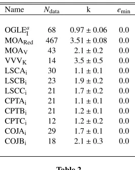
Name Ndata k emin
OGLEa
I 68 0.97±0.06 0.0
MOARed 467 3.51±0.08 0.0
MOAV 43 2.1±0.2 0.0
VVVK 14 3.5±0.5 0.0
LSCAi 30 1.1±0.1 0.0
LSCBi 23 1.9±0.2 0.0
LSCCi 21 1.7±0.2 0.0
CPTAi 21 1.1±0.1 0.0
CPTBi 21 1.2±0.1 0.0
CPTCi 12 1.2±0.2 0.0
COJAi 29 1.7±0.1 0.0
[image:3.612.372.505.264.431.2]COJBi 18 2.1±0.3 0.0
Table 2
Error bar rescaling coefficients used in this paper.aNote that the OGLE
I
uncertainties receive a special treatment before this rescaling step, see text. As a secondary check, we follow the same approach as Do-minik et al. (2018) and fit the parameters of Equation 1 around the best model from the previous section, using the modified χ20:
χ20=X
i
(fi−mi)2 σ02
i
+2 ln(σ0i) (2)
with fi the observed flux,mithe microlensing model in flux
andσ0
iis the modified error in flux relative to Equation 1. It
appeared rapidly that the termeminwas not constrained, due to the relative small range of magnification in the light curves. We therefore delete this term from Equation 1 and fit only the first termk. The results presented in the Table 2 are consistent with the previous analysis and indicate a soft rescaling, with the exception of the MOAReddataset.
3.3. Results
Both algorithms converged to models with similar geome-tries: the strong anomalies seen in Figure 1 are due to a central caustic crossing. However the data do not constrain strongly the models, leading to significant difference in the model pa-rameters given in the Table 3. To obtain a more comprehen-sive picture, we run two sets of Monte-Carlo Markov Chain (MCMC) explorations around these best models, using the
in pyLIMA. Note that during this optimization process, we modified the model parameters so that we modeltc anduc,
the time and closest approach to the central caustic, instead of t0andu0. The idea is to use parameters more directly related to the main features of the light curve. This is a standard prac-tice that significantly improves the model convergence (Cas-san 2008; Han 2009; Penny 2014).
The geometry of the best fitting model is sensitive to the close/wide degeneracy (Griest & Safizadeh 1998; Bozza 2000; Dominik 2009). However, close models are slightly fa-vored. The mass ratio of this event is not well constrained. This is due to a lack of observations during the anomaly, es-pecially during the central caustic entrance and exit.
We tried to model second-order effects, such as annual par-allax and the orbital motion of the lens (Gould & Loeb 1992; Dominik 1998; Albrow et al. 2000; Gould 2004; Bachelet et al. 2012b). Due to the relatively short timescale of the event and the relatively low coverage of the anomaly features, these second order effects were not constrained well enough to be considered as a solid detection.
4. PROPERTIES OF THE SOURCE
4.1. Optical observations
Following Bond et al. (2017), we calibrated the MOAR and MOAVmagnitudes to the OGLEIIIsystem using the rela-tion in the Appendix. The resulting color-magnitude diagram (CMD thereafter) is presented in Figure 2, and we summa-rize information from the various catalogs used in Table 4. We found that the color of the red giant clump (RGC) cen-troid is (V −I)RGC = 1.75±0.05 mag and its brightness is IRGC = 15.3±0.1 mag. Knowing the intrinsic color of the RGC (V −I)0,RGC = 1.06 mag and its intrinsic brightness I0,RGC =14.45 mag (Nataf et al. 2013), we estimate the ab-sorptionAI = 0.9±0.1 mag and the extinction E(V −I) =
0.69±0.05 mag toward the microlensing event. We found a good agreement with an independent determination using the Interstellar Extinction Calculator on the OGLE website3, based on Nataf et al. (2013) and Gonzalez et al. (2012), with AI =0.79±0.1 mag andE(V−I)=0.68±0.05 mag. From
the best model and the color transformations in the Appendix, the source magnitudes are Vs,OGLEIII = 21.2±0.1 mag and
Is,OGLEIII =19.15±0.09 mag (and a color of (V−I)s,OGLEIII = 2.0±0.1 mag). In principle, it is possible to obtain a model-independent color using linear regression between two bands λ1andλ2since the microlensing magnification is achromatic (Dong et al. 2006; Bond et al. 2017):
fλ1=
fs,λ1 fs,λ2
(fλ2−fb,λ2)+fb,λ1 (3) where fs and fb are the source and blending flux
respec-tively. However, this requires simultaneous observations which are difficult in practice. Here, we consider MOARand MOAV as simultaneous if the acquisition time was within 15 minutes. We found a model independent source color of (V −I)s,OGLEIII = 2.0±0.1 mag, in agreement with the previous estimation. Finally, we obtained the intrisic color (V−I)o,s,OGLEIII =1.4±0.1 mag and brightnessIo,s,OGLEIII = 18.4±0.1 of the source in the OGLE-III system (i.e., in the Johnson-Cousins system).
Because this event was also observed by OGLE-IV, we con-ducted a similar analysis using the OGLE-IV CMD. The
cor-3http://ogle.astrouw.edu.pl/
responding CMD is presented in Figure 2. In this CMD, we found that the color of the red giant clump (RGC) cen-troid is (V −I)RGC = 1.67±0.05 mag and its brightness is IRGC = 15.3±0.1 mag. The best model and theV-band transformation in Equation A4 lead toVs,OGLEIV =21.2±0.1 mag and Is,OGLEIV = 19.47 ±0.01 mag (and a color of (V−I)s,OGLEIV =1.7±0.1 mag). Assuming the source suffers the same extinction as the RGC, we measured an offset be-tween the source and the RGC∆((V−I)s,OGLEIV,Is,OGLEIV)= (0.03±0.1,4.2±0.1). However, the OGLE-IV system is not perfectly calibrated, and the difference in the colors need to be multiplied by a factor 0.93 (for the CCD 24 of the OGLE camera mosaic) (Udalski et al. 2015). Based on the OGLE-IV CMD, the source color is (V−I)o,s,OGLEIV =1.09±0.1 mag and the brightness isIo,s,OGLEIV =18.7±0.1 mag.
While the two studies converge to a similar conclusion, we use for the source properties (V −I)o,s,OGLEIV = 1.09±0.1 mag andIo,s,OGLEIV =18.7±0.1 mag, because they rely on a single color transformation and also because the color term in Equation A4 is smaller than the one in Equation A2. From op-tical observations, the source is probably a K-dwarf (Bessell & Brett 1988) or, potentially, a K subgiant that lies behind the Galactic Bulge.
Using Kervella & Fouqu´e (2008) and the optical color, we can obtain the angular source radiusθ∗. We obtain 13%
preci-sion onθ∗=0.8 ±0.1µas. Finally, we can then estimate the
angular Einstein ring radiusθE =θ∗/ρ=0.8±0.2 mas (using
the best model) andµ = 7.0±3 mas/yr. This provides one mass and distance constraint to the lens system since (Gould 2000):
Mtot=
θ2
E κπrel
(4)
withπrel= 1D−x
sxau,x=Dl/Ds(the distance to the lens and the source respectively) and the constantκ=8.144 mas.M−1.
4.2. Near infrared
Thanks to VVV observations, we can perform a similar study usingK-band data and construct a near-infrared CMD, as shown in Figure 3. Gonzalez et al. (2012) provide ex-tinction maps toward the Galactic Bulge. Using their online tool 4, we found A
K = 0.10±0.06 mag and E(J −K) =
0.19±0.11 mag. This agrees relatively well with the 3D Maps toward the Galactic Bulge of Schultheis et al. (2014) (i.e.,E(J−K)=0.30±0.06 mag andAK =0.16±0.04 mag
assuming Nishiyama et al. (2009) extinction law). From the best model, the source brightness isKs,s=17±1 mag and the
blend brightness isKs,b =13.61±0.03 mag. The relatively
low precision on the source magnitude inKsis again due to
the lack of observations during the event high-magnification pahse of the event. Unfortunately, the maximum observed magnification was only A ∼ 1.6, while the secondary maxi-mum observed magnification wasA∼1.05. The color of the source is (IOGLEIV−KVVV)=2±1 mag, leading to an extinc-tion corrected color of (IOGLEIV−KVVV)o=2.0−AI+AK =1±1 mag, and a magnitude ofK0,VVV=17±1 mag. Using Bessell & Brett (1988), we found that this color is consistent with the optical colour and corresponds to a K-type source star.
4.3. Does the source belong to the Sagittarius Dwarf
Galaxy?
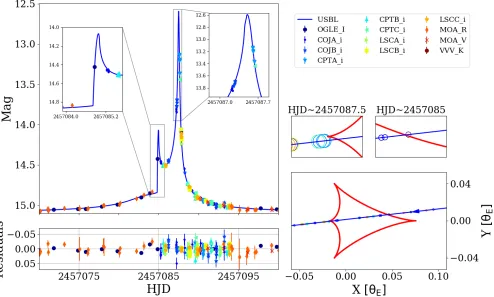
Figure 1.Left: Light curves and best-fit model for OGLE-2015-BLG-0232.Right: Central caustic (red curve), source trajectory (blue line), and source positions at the epoch of observations. The insets show zooms around the caustic crossings. There was one OGLEImeasurement during the caustic entry and four CPTAi
points (only two are visible in the inset) during the cusp exit. This allows a reasonable constraint on the normalised source radiusρ.
Parameters pyLIMA (s<1) RT Model†(s<1) MCMC(s<1) pyLIMA (s>1) RT Model†(s>1) MCMC(s>1)
tc−2450000 7087.20(1) 7087.49(4) 7087.2(2) 7086.68(4) 7086.93(4) 7086.76(8)
uc -0.00048(4) 0.00135(7) -0.0005(6) 0.00320(8) 0.0020(2) 0.0026(5)
tE 41.7(3) 46.1(3) 42(6) 34.7(1) 35(3) 39(3)
ρ(10−4) 9.9(3) 19.9(8) 10(1) 7.0(5) 7.0(2) 7.3(9)
s 0.545(2) 0.699(2) 0.55(7) 3.05(1) 2.58(2) 2.9(2)
q 0.0597(8) 0.0180(1) 0.06(2) 0.338(3) 0.17(1) 0.24(6)
α -3.031(3) -3.061(2) -3.03(2) 3.017(4) 3.045(5) 3.008 (9)
χ2 766 799 764 822 843 812
†The parameters are obtained from the online RTModel website (http://www.fisica.unisa.it/gravitationAstrophysics/RTModel/2015/RTModel.htm). Table 3
Close/Wide best models of pyLIMA, RTModel and MCMC explorations. Models from RTModel were used as starting point for a Levenberg-Marquardt (LM) optimization with pyLIMA. Numbers in bracket in the table represents 1σerrors from LM and 68% range for the MCMC explorations.
Due to the relatively large galactic latitude of the event (i.e, b = −5◦.9060), the line of sight does not go through much of the Galactic Disk. This raises the possibility that the source is located in the stream of the Sagittarius Dwarf galaxy (Ibata et al. 1994). If this were the case, the source would be located very far away, Ds ∼ 25 kpc. Cseresnjes
& Alard (2001) predicted that events due to the Sagittarius dwarf galaxy should represent roughly 1% of the total events detected toward the Galactic Bulge fields each year. They also predicted that these events should mainly occur for main-sequence source stars withV ≥21 mag and that the median Einstein ring radius crossing time would be 1.3 times larger than the one observed for Milky Way sources. To test this, we constructed a map of the Sagittarius Dwarf galaxy in Fig-ure 4. We followed the method of Majewski et al. (2003) and
selected stars withE(B−V)<0.555, 0.95<(J−Ks)o<1.10
and 10.5 < Ks,o < 12 combined with the extinction maps
from Schlegel et al. (1998) (with a low resolution of 0.5 deg)5. However, the line of sight (`=−1◦.17,b=−5◦.90) is quite distant from the highest density of the Sagittarius Dwarf galaxy: M54. The Sagittarius dwarf star population has been studied in great detail, see for example Marconi et al. (1998); Monaco et al. (2002, 2004); Giuffrida et al. (2010). Sev-eral features can be used to distinguish stars from the Milky Way and the dwarf galaxy. In particular, the CMD of the dwarf galaxy presents several horizontal branches and red-giant branches, signatures of different star populations. The
5 We use the python implementation available at
[image:5.612.89.520.411.520.2]Figure 2. Optical color-magnitude diagrams of stars within 2’ of the line of sight of this event. OGLE and the transformed MOA are in blue (filled and empty respectively), the source is in red, the blend is in orange, and the position of the RGC is in magenta. The star symbol represents the star presented in the Table 4. The grey squares represent the region used to estimate the position of the RGC. Left :OGLEIIIphotometric system (i.e, Johnson-Cousins (Szyma´nski et al. 2011)).
Right: instrumental OGLEIVphotometric system.
Figure 3. Color magnitude diagram of stars within 2’ of the line of sight to
this event, using IOGLEIVand KVVV.
optical CMD of OGLE-2015-BLG-0232 does not show these signatures, indicating that there is no significant contamina-tion from the dwarf galaxy.
Due to the large distance to the center of the Sagittarius Dwarf galaxy (≥ 10◦) and the absence of particular features
in the CMD, we discount this hypothesis and assume that the source star belongs to the Milky Way.
5. INFORMATION ON THE BLEND
[image:6.612.325.562.327.519.2]Results from our modeling indicate that this event was highly blended. It is clear from Figure 2 and Figure 3 that the blend belongs to the foreground stars branch of the CMD, in-dicating a close blend. In the following, we consider the blend as a single star and neglect the potential contamination from the source because the blend ratio is substantial withg∼50.
Figure 4. Map of the Sagittarius Dwarf galaxy from the 2MASS catalog
(Cutri et al. 2003; Skrutskie et al. 2006).
5.1. Gaia measurements
The Gaia mission (Gaia Collaboration et al. 2016, 2018; Luri et al. 2018) recently released a vast catalog of paral-lax and proper motions measurements for more than a billion of stars. In addition to this goldmine, effective temperatures, radii and luminosities are also estimated. We summarized the Gaia measurements for OGLE-2015-BLG-0232 in Table 4. Recent studies indicate biases in Gaia parallax measurements of severalµas (Lindegren et al. 2018; Zinn et al. 2018; Riess et al. 2018). We therefore use the estimation of the blend distanceDb =1023+−8675 pc by Bailer-Jones et al. (2018), and
so the blend is a late-type G or an early-type K dwarf. For this target, we also foundTeff =4707+−269228K,R =1.0+−00..11 R,
L = 0.42+0.07
−0.07L and ultimately estimated the mass of this blend M ∼ L1/4 ∼ 0.8M
, typical of a K-dwarf. However,
[image:6.612.58.286.344.553.2]ap-proximation is reasonable for this target because the blend is relatively close and the extinction along the line of sight is relatively small, these fundamental parameters are probably biased.
The brightnesses of the blend in the Gaia bands areG = 15.918±0.001 mag, GBP = 16.48±0.01 mag andGRP =
15.15±0.01 mag. Using the system transformation in the Ap-pendix, we convert these magnitudes to the Johnson-Cousins system to findV =16.25±0.05 mag andI=15.08±0.05 mag. Given the blend distance, we assumed half extinction and found an intrinsic color (V−I)o,b,G=1.33−0.69/2=1.0±0.1
and brightnessIo,b,G=15.08−0.79/2=14.7±0.1 mag,
typi-cal of a K2 dwarf star (Bessell & Brett 1988). Using the color-effective temperature relation of Casagrande et al. (2010), the blend effective temperature isTeff = 4900±400 K. We es-timated the blend physical radiusRb =0.8±0.1R, the
lu-minosityL=0.3±0.1Land finally derived the blend mass Mb∼0.7M(Boyajian et al. 2012). Knowing that the angular
radius of the blend isθb =4.8±0.5µas(Kervella & Fouqu´e
2008), one can derive an indepedent estimate of the blend dis-tanceDb =800±200 pc, in good agreement with the Gaia
parallax measurement.
If the blend were the lens and assuming that the source is at 8 kpc, a blend mass ofMb ∼0.7Mat a distanceDb∼1000
pc, the angular Einstein ring would beθE,b∼2.2 mas. This is
in strong disagreement with the value ofθE =0.8±0.2 mas
derived in Section 4.1. This is a first clue that the bright blend is likely not the lens.
From Table 4, the proper motion of the bright blend is µG(N,E)=(2.2±0.1,9.9±0.1) mas/yr. The speed of the Sun
in the Galactic frame isV(U,V,W)∼(11,12,7)+(0,220,0)
km/s (Fich et al. 1989; Sch¨onrich et al. 2010): the first term is the intrinsic Sun velocity and the second term is the speed of the Galactic disk in the Galactic coordinates system. Assum-ing the source is at 8 kpc, the expected proper motion of the source is aboutµs(l,b)∼(−6±3,0±3) mas/yr, see Kuijken
& Rich (2002) and Kozłowski et al. (2006) for the estimation of the uncertainties. The Galactic proper motion transform toµs(α, δ) ∼(−3±3,−5±3) mas/yr (Binney & Merrifield
1998; Poleski 2013; Bachelet et al. 2018). Therefore, if the bright blend were the lens, one would expect a relative proper motion ofµrel(N,E)= µs−µG ∼(−5±3,−15±3) mas/yr.
The relative proper motion would beµrel=16±4 mas/yr, in
disagreement with the estimationµrel =7±3 mas/yr of the
Section 4.1. This is the second clue that the blend is not the lens.
5.2. Blend brightness from models
Using our best-fit model and the color relationships given in the Appendix, we derived the brightnesses of the blend: Ib,OGLEIV =15.1163±0.0007 mag, Vb,OGLEIV =16.23±0.08 mag and Kb,VVV=13.61±0.03 mag. Assuming that the blend suffers half the extinction, we found that the blend brightness isIo,b,OGLEIV =14.7±0.1 mag and the blend color is (IOGLEIV−
KVVV)o,b =1.1±0.1 mag, consistent with its being an early
K-dwarf (Bessell & Brett 1988). This is in good agreement with the Gaia measurements.
5.3. Astrometry
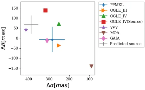
[image:7.612.319.566.73.227.2]Toward the Galactic Bulge and for stellar masses, mi-crolensing occurs when the alignement between the lens and the source is less than a few mas. We therefore compared the position of centroids between the baseline object and the
Figure 5. Location of the target from the catalogs listed in the Table 4,
cen-tered at (RA=271.6826◦, DEC=−32.9076◦) (J2000). North is up and East is left. Some uncertainties have been hidden for clarity. The source position measured from OGLE-IV is located at∆(E,N)=(78,78) mas (red square) from the OGLE-IV position. The grey cross indicates the predici-ton of the source, applying the offset to the Gaia position and assuming
σ(N,E)=(45,35) mas uncertainties.
magnified source from the OGLE-IV images. In pixel co-ordinates, the magnified source has an offset of ∆(N,E) = (78±45,78±35) mas from the bright blend centroid (the precision of the bright blend centroid is about 0.05 pixel, i.e. σ(N,E) = (13,13) mas). The two positions are different enough (i.e., 1.5σ) to assume that this is the third clue that the blend is likely not the lens.
5.4. The lens as a blend companion
In the following, we explore the possibility that the lens is a companion of the blend. From the astrometry offset de-rived in Section 5.3, we can derive the separation δ of the blend with its potential companion and foundδ = 110 mas, which corresponds to aproj ∼ 110 au at 1 kpc. If this po-tential companion is indeed a component of the lens system, then the mass ratio between the binary blend components is qb = (θE/θE,b)2 = (0.8/2.2)2 ∼ 0.13, leading to a potential
companion mass of Mb,2 = 0.13×0.7 ∼ 0.1M.
There-fore, such a companion is not bright enough to have been significantly detected. Because the normalised separation be-tween the putative companion and the bright blend is impor-tant sb = 110/2.2 ∼ 50, the hypothetic companion blend
could have acted as a binary lens and left no signature of a triple-lens, as observed. However, this hypothetic companion would have a similar proper motion as the bright blend and the analysis on the relative proper motions in Section 5.1 also ap-ply here. Therefore, the lens as a blend companion hypothesis is unlikely.
6. DISCUSSION AND POTENTIAL NEW CLUES
All available information seem to concur that the blend light is mainly due to a close K dwarf. Both astrometry and the con-straint from finite-source effects reject the hypothesis that the bright blend is the lens. The light of the lens is not signifcantly detected and there are no constraints from the microlensing parallax: the distance and exact nature of the lens remains un-certain at the present time. However, considering a large mass range for the lens primaryMl,1∈[0.1,2.0]M(corresponding
toDl ≤5.5 kpc according to Equation 4 andθE =0.8±0.2
mas), the companion mass range isMl,2∈[6,130]MJup. The
Catalog Source ID Epoch RA(J2000) DEC(J2000) Parallax µα µδ
◦ ◦
mas mas/yr mas/yr Gaia 4042761215742767360 J2015.5 271.68268633(1) -32.90760309(1) 0.96(7) 9.9(1) 2.0(1)
MOA 965 - 271.68263(4) -32.90764(3) - -
-OGLE-III 90793 J2002.46 271.68267(4) -32.90761(3) - -
-OGLE-IV (baseline) 58780 J2011.4 271.68267(4) -32.90758(3) - -
-OGLE-IV (source) - J2011.4 271.68269(4) -32.90720(3) - -
-VVV 2508 J2010 271.68262 -32.90763 - -
-PPMXL 4938889137283654706 J1991.21 271.68268(2) -32.90760(2) - 10.6(5.2) 6.3(5.2)
Table 4
Astrometry of the target in MOA, OGLE-III, OGLE-IV, VVV and Gaia catalogs. OGLE-III catalog of the field is from Szyma´nski et al. (2011). OGLE-IV catalog is available onlinea. VVV catalog is from Beaulieu et al. (2016). The PPMXL catalog is from Roeser et al. (2010). Numbers in parenthesis are the 1σ
or a low-mass M-dwarf if Dl ≤ 5.5 kpc. It the lens is more
distant, the primary is probably a stellar remnant, otherwise the lens light would have been detected. This indicates the need for supplementary observations to reveal the nature of the lens OGLE-2015-BLG-0232.
High-resolution imaging is an important tool for microlens-ing. Several planets have been confirmed using space or ground-based facilities and had their measured properties re-fined, see for example (Batista et al. 2015; Bennett et al. 2015; Beaulieu et al. 2017). High-resolution imaging is useful for two reasons. First, it is possible to estimate the source-lens proper motionµfrom high-resolution images obtained several years after the microlensing event, when the source and the lens are well separated (Batista et al. 2015). High-resolution imaging can also provide measurements of source and, some-times, lens fluxes and therefore tightly constrain the mass-distance relation of the lens (Ranc et al. 2015; Batista et al. 2015; Bennett et al. 2015; Beaulieu et al. 2017).
In the case of OGLE-2015-BLG-0232, high-resolution imaging will contribute to confirming/rejecting scenarios and possibly estimate the mass of the lens. The first step will be to challenge the assumption that the blend is a single star. This can be done immediately. Moreover, one can predict a more precise source position based on Gaia astrometry and the mea-sured offset from the OGLE-IV photometry. The predicted position of the source is shown in the Figure 5, assuming 26 mas precision on OGLE-IV measurement (i.e., 0.1 pixel). The comparison of the flux at this position in high resolution im-ages with the measured source fluxes from models could place constraints on the nature of the lens.
A second step will be to wait several years for the bright blend leaves the line of sight to obtain more information on the source/lens system. Because µb = 11 ±0.2 mas/yr,
the blend is separating faster than the lens/source system µ =7.0±3 mas/yr. In a decade, the blend should be about 11 pixels away from the line of sight while the source and the lens separation should be about 7 pixel (for a typical high-resolution pixel scale of 10 mas/pix).
Low-resolution spectroscopy could also confirm the spec-tral type of the bright blend. Similarly, the study of emission/absorption lines with high-resolution spectroscopy would allow a precise understanding of the blend. Finally, one could combine spectroscopic and photometric informa-tion to explore various scenarios in a Bayesian analayis (San-terne et al. 2016).
7. CONCLUSION
We presented an analysis of the binary microlensing event OGLE-2015-BLG-0232. Because the event occurred during full moon, the observations do not constrain much the devia-tions from the single-lens model. However, results from the modeling favor a close brown dwarf companion (i.e.,s∼0.55 andq ∼ 0.06). The source is estimated to be red and faint, probably a K dwarf in the Galactic Bulge. We also tested, and ultimately rejected, the hypothesis that the source belongs to the Sagittarius Dwarf Galaxy. Since the microlensing
paral-lax is not measured, we obtain only one (weak) constraint, from finite-source effects, on the mass and distance of the lens. Based on the recent Gaia DR2 release and OGLE-IV astrometry, we were able to infer that the bright blend is a K dwarf at 1 kpc and is most likely not the lens. We finally discuss the potential of additional observations to confirm the nature of the blend and ultimately to derive the exact nature of the lens.
ACKNOWLEDGEMENTS
The authors thank the anonymous referee for the construc-tive comments. This research has made use of NASA’s As-trophysics Data System. Work by EB and RAS is sup-port by the NASA grant NNX15AC97G. Work by C. Han was supported by the grant (2017R1A4A1015178) of Na-tional Research Foundation of Korea. This work makes use of observations from the LCOGT network. The OGLE project has received funding from the National Science Cen-tre, Poland, grant MAESTRO 2014/14/A/ST9/00121 to AU. The MOA project is supported by JSPS KAKENHI Grant Number JSPS24253004, JSPS26247023, JSPS23340064, JSPS15H00781, JP16H06287 and JP17H02871. The work by C.R. was supported by an appointment to the NASA Postdoctoral Program at the Goddard Space Flight Cen-ter, administered by USRA through a contract with NASA. This work has made use of data from the European Space Agency (ESA) mission Gaia(https://www.cosmos.esa. int/Gaia), processed by theGaiaData Processing and Anal-ysis Consortium (DPAC,https://www.cosmos.esa.int/ web/Gaia/dpac/consortium). Funding for the DPAC has been provided by national institutions, in particular the insti-tutions participating in theGaiaMultilateral Agreement. This publication makes use of data products from the Two Micron All Sky Survey, which is a joint project of the University of Massachusetts and the Infrared Processing and Analysis Center/California Institute of Technology, funded by the Na-tional Aeronautics and Space Administration and the NaNa-tional Science Foundation. This research made use of Astropy, a community-developed core Python package for Astronomy (Astropy Collaboration, 2013). This research has made use of the SIMBAD database, operated at CDS, Strasbourg, France. The DENIS project has been partly funded by the SCIENCE and the HCM plans of the European Commission under grants CT920791 and CT940627. It is supported by INSU, MEN and CNRS in France, by the State of Baden-W¨urttemberg in Germany, by DGICYT in Spain, by CNR in Italy, by FFwBWF in Austria, by FAPESP in Brazil, by OTKA grants F-4239 and F-013990 in Hungary, and by the ESO C&EE grant A-04-046. Jean Claude Renault from IAP was the Project manager. Observations were carried out thanks to the con-tribution of numerous students and young scientists from all involved institutes, under the supervision of P. Fouqu´e, sur-vey astronomer resident in Chile. DPB, AB, and CR were supported by NASA through grant NASA-80NSSC18K0274.
APPENDIX
COLOR TRANSFORMATIONS
In this work, we used several color transformations that we summarize here. First, we calibrated the MOA instrumental magnitudes to the OGLE-III catalog (Udalski 2003; Bond et al. 2017) using the relationships :
VOGLEIII =VMOA+(28.556±0.002)+(−0.164±0.002)(VMOA−RMOA)±0.08 (A2) We also calibrated the MOA instrumental magnitudes to the OGLE-IV system using:
IOGLEIV =RMOA+(27.990±0.003)+(−0.247±0.009)(VMOA−RMOA)±0.08 (A3)
VOGLEIV =VMOA+(28.425±0.005)+(−0.062±0.006)(VMOA−RMOA)±0.08 (A4) We also used the transformation of the 2MASS colors into the the VVV system (Soto et al. 2013):
JVVV=J2MASS−0.077(J2MASS−H2MASS) (A5)
HVVV=H2MASS+0.032(J2MASS−H2MASS) (A6)
KVVV=K2MASS+0.010(J2MASS−K2MASS) (A7)
Transformations into the Bessell & Brett photometric system (Bessell & Brett 1988) are the revised version6 of Carpenter (2001):
(Ks)2MASS=KBB+(−0.039±0.007)+(0.001±0.005)(J−K)BB (A8) (J−Ks)2MASS=(−0.018±0.007)+(0.001±0.005)(J)BB (A9) Finally, the transformation of the Gaia DR2 to the Johnson-Cousins system is available online7:
G−VJC=−0.01760−0.006860(GBP−GRP)−0.1732(GBP−GRP)2±0.045858 (A10) G−IJC=0.02085+0.7419(GBP−GRP)−0.096311(GBP−GRP)2±0.04956 (A11)
REFERENCES
Albrow, M. D., Beaulieu, J.-P., Caldwell, J. A. R., et al. 2000, ApJ, 535, 176 Albrow, M. D., Horne, K., Bramich, D. M., et al. 2009, MNRAS, 397, 2099 Andrae, R., Fouesneau, M., Creevey, O., et al. 2018, A&A, 616, A8 Andrae, R., Schulze-Hartung, T., & Melchior, P. 2010, ArXiv e-prints Bachelet, E., Beaulieu, J.-P., Boisse, I., Santerne, A., & Street, R. A. 2018,
ArXiv e-prints
Bachelet, E., Bramich, D. M., Han, C., et al. 2015, ApJ, 812, 136 Bachelet, E., Fouqu´e, P., Han, C., et al. 2012a, A&A, 547, A55 Bachelet, E., Norbury, M., Bozza, V., & Street, R. 2017, AJ, 154, 203 Bachelet, E., Shin, I.-G., Han, C., et al. 2012b, ApJ, 754, 73
Bailer-Jones, C. A. L., Rybizki, J., Fouesneau, M., Mantelet, G., & Andrae, R. 2018, AJ, 156, 58
Batista, V., Beaulieu, J.-P., Bennett, D. P., et al. 2015, ApJ, 808, 170 Beaulieu, J.-P., Batista, V., Bennett, D. P., et al. 2017, ArXiv e-prints Beaulieu, J.-P., Bennett, D. P., Batista, V., et al. 2016, ApJ, 824, 83 Bennett, D. P., Bhattacharya, A., Anderson, J., et al. 2015, ApJ, 808, 169 Bessell, M. S. & Brett, J. M. 1988, PASP, 100, 1134
Binney, J. & Merrifield, M. 1998, Galactic Astronomy Bond, I. A., Abe, F., Dodd, R. J., et al. 2001, MNRAS, 327, 868 Bond, I. A., Bennett, D. P., Sumi, T., et al. 2017, MNRAS, 469, 2434 Bonfils, X., Delfosse, X., Udry, S., et al. 2013, A&A, 549, A109 Boyajian, T. S., von Braun, K., van Belle, G., et al. 2012, ApJ, 757, 112 Bozza, V. 2000, A&A, 359, 1
Bozza, V. 2010, MNRAS, 408, 2188
Bozza, V., Dominik, M., Rattenbury, N. J., et al. 2012, MNRAS, 424, 902 Bramich, D. M. 2008, MNRAS, 386, L77
Bramich, D. M., Horne, K., Albrow, M. D., et al. 2013, MNRAS, 428, 2275 Bryan, M. L., Benneke, B., Knutson, H. A., Batygin, K., & Bowler, B. P.
2018, Nature Astronomy, 2, 138
Buchhave, L. A., Latham, D. W., Johansen, A., et al. 2012, Nature, 486, 375 Burrows, A., Hubbard, W. B., Lunine, J. I., & Liebert, J. 2001, Reviews of
Modern Physics, 73, 719
Burrows, A. & Liebert, J. 1993, Reviews of Modern Physics, 65, 301 Carpenter, J. M. 2001, AJ, 121, 2851
Casagrande, L., Ram´ırez, I., Mel´endez, J., Bessell, M., & Asplund, M. 2010, A&A, 512, A54
Cassan, A. 2008, A&A, 491, 587
Cassan, A., Kubas, D., Beaulieu, J.-P., et al. 2012, Nature, 481, 167 Chung, S.-J., Zhu, W., Udalski, A., et al. 2017, ApJ, 838, 154 Clanton, C. & Gaudi, B. S. 2016, ApJ, 819, 125
Cseresnjes, P. & Alard, C. 2001, A&A, 369, 778
Cutri, R. M., Skrutskie, M. F., van Dyk, S., et al. 2003, VizieR Online Data Catalog, 2246
Dominik, M. 1998, A&A, 329, 361
Dominik, M. 1999, A&A, 349, 108 Dominik, M. 2009, MNRAS, 393, 816
Dominik, M., Bachelet, E., Bozza, V., et al. 2018, ArXiv e-prints Dominik, M., Rattenbury, N. J., Allan, A., et al. 2007, MNRAS, 380, 792 Dong, S., DePoy, D. L., Gaudi, B. S., et al. 2006, ApJ, 642, 842 Erdl, H. & Schneider, P. 1993, A&A, 268, 453
Fich, M., Blitz, L., & Stark, A. A. 1989, ApJ, 342, 272
Foreman-Mackey, D., Hogg, D. W., Lang, D., & Goodman, J. 2013, PASP, 125, 306
Fressin, F., Torres, G., Charbonneau, D., et al. 2013, ApJ, 766, 81 Gaia Collaboration, Brown, A. G. A., Vallenari, A., et al. 2018, ArXiv
e-prints
Gaia Collaboration, Prusti, T., de Bruijne, J. H. J., et al. 2016, A&A, 595, A1 Giuffrida, G., Sbordone, L., Zaggia, S., et al. 2010, A&A, 513, A62 Gonzalez, O. A., Rejkuba, M., Zoccali, M., et al. 2012, A&A, 543, A13 Gould, A. 2000, ApJ, 542, 785
Gould, A. 2004, ApJ, 606, 319
Gould, A. & Loeb, A. 1992, ApJ, 396, 104 Griest, K. & Safizadeh, N. 1998, ApJ, 500, 37 Han, C. 2009, ApJ, 691, L9
Han, C., Jung, Y. K., Udalski, A., et al. 2016, ApJ, 822, 75
Hundertmark, M., Street, R. A., Tsapras, Y., et al. 2017, ArXiv e-prints Ibata, R. A., Gilmore, G., & Irwin, M. J. 1994, Nature, 370, 194 Kervella, P. & Fouqu´e, P. 2008, A&A, 491, 855
Kozłowski, S., Wo´zniak, P. R., Mao, S., et al. 2006, MNRAS, 370, 435 Kuijken, K. & Rich, R. M. 2002, AJ, 124, 2054
Latham, D. W., Stefanik, R. P., Torres, G., et al. 2002, AJ, 124, 1144 Liebig, C., D’Ago, G., Bozza, V., & Dominik, M. 2015, MNRAS, 450, 1565 Lindegren, L., Hern´andez, J., Bombrun, A., et al. 2018, A&A, 616, A2 Luri, X., Brown, A. G. A., Sarro, L. M., et al. 2018, ArXiv e-prints Majewski, S. R., Skrutskie, M. F., Weinberg, M. D., & Ostheimer, J. C.
2003, ApJ, 599, 1082
Mao, S. & Di Stefano, R. 1995, ApJ, 440, 22
Marconi, G., Buonanno, R., Castellani, M., et al. 1998, A&A, 330, 453 Minniti, D., Lucas, P. W., Emerson, J. P., et al. 2010, New A, 15, 433 Miyake, N., Udalski, A., Sumi, T., et al. 2012, ApJ, 752, 82
Monaco, L., Bellazzini, M., Ferraro, F. R., & Pancino, E. 2004, MNRAS, 353, 874
Monaco, L., Ferraro, F. R., Bellazzini, M., & Pancino, E. 2002, ApJ, 578, L47
Mordasini, C., Alibert, Y., Benz, W., Klahr, H., & Henning, T. 2012, A&A, 541, A97
Mortier, A., Santos, N. C., Sozzetti, A., et al. 2012, A&A, 543, A45 Mr´oz, P., Han, C., and, et al. 2017, AJ, 153, 143
Nataf, D. M., Gould, A., Fouqu´e, P., et al. 2013, ApJ, 769, 88
Nishiyama, S., Tamura, M., Hatano, H., et al. 2009, ApJ, 696, 1407 Penny, M. T. 2014, ApJ, 790, 142
Poleski, R. 2013, ArXiv e-prints
Poleski, R., Udalski, A., Bond, I. A., et al. 2017, A&A, 604, A103 Ranc, C., Cassan, A., Albrow, M. D., et al. 2015, A&A, 580, A125 Riess, A. G., Casertano, S., Yuan, W., et al. 2018, ApJ, 861, 126 Roeser, S., Demleitner, M., & Schilbach, E. 2010, AJ, 139, 2440 Santerne, A., Beaulieu, J.-P., Rojas Ayala, B., et al. 2016, A&A, 595, L11 Schlaufman, K. C. 2018, ApJ, 853, 37
Schlegel, D. J., Finkbeiner, D. P., & Davis, M. 1998, ApJ, 500, 525 Schneider, J., Dedieu, C., Le Sidaner, P., Savalle, R., & Zolotukhin, I. 2011,
A&A, 532, A79
Sch¨onrich, R., Binney, J., & Dehnen, W. 2010, MNRAS, 403, 1829 Schultheis, M., Chen, B. Q., Jiang, B. W., et al. 2014, A&A, 566, A120 Shvartzvald, Y., Yee, J. C., Skowron, J., et al. 2018, ArXiv e-prints Skowron, J., Udalski, A., Kozłowski, S., et al. 2016, Acta Astron., 66, 1 Skrutskie, M. F., Cutri, R. M., Stiening, R., et al. 2006, AJ, 131, 1163 Soto, M., Barb´a, R., Gunthardt, G., et al. 2013, A&A, 552, A101
Spiegel, D. S., Burrows, A., & Milsom, J. A. 2011, ApJ, 727, 57 Storn, R. & Price, K. 1997, J. of Global Optimization, 11, 341 Suzuki, D., Bennett, D. P., Sumi, T., et al. 2016, ApJ, 833, 145
Szyma´nski, M. K., Udalski, A., Soszy´nski, I., et al. 2011, Acta Astron., 61, 83
Tsapras, Y., Street, R., Horne, K., et al. 2009, Astronomische Nachrichten, 330, 4
Udalski, A. 2003, Acta Astron., 53, 291
Udalski, A., Szyma´nski, M. K., & Szyma´nski, G. 2015, Acta Astron., 65, 1 Wright, J. T., Fakhouri, O., Marcy, G. W., et al. 2011, PASP, 123, 412 Yee, J. C., Hung, L.-W., Bond, I. A., et al. 2013, ApJ, 769, 77 Zapolsky, H. S. & Salpeter, E. E. 1969, ApJ, 158, 809 Zhu, W., Calchi Novati, S., Gould, A., et al. 2016, ApJ, 825, 60 Zinn, J. C., Pinsonneault, M. H., Huber, D., & Stello, D. 2018, ArXiv