A review of methods for the calculation of solution free energies and the modelling of systems in solution

(1)

Cite this:DOI: 10.1039/c5cp00288e

A review of methods for the calculation

of solution free energies and the modelling

of systems in solution

R. E. Skyner,†aJ. L. McDonagh,†aC. R. Groom,bT. van Mourikaand J. B. O. Mitchell*a

Over the past decade, pharmaceutical companies have seen a decline in the number of drug candidates successfully passing through clinical trials, though billions are still spent on drug development. Poor aqueous solubility leads to low bio-availability, reducing pharmaceutical eﬀectiveness. The human cost of ineﬃcient drug candidate testing is of great medical concern, with fewer drugs making it to the production line, slowing the development of new treatments. In biochemistry and biophysics, water mediated reactions and interactions within active sites and protein pockets are an active area of research, in which methods for modelling solvated systems are continually pushed to their limits. Here, we discuss a multitude of methods aimed towards solvent modelling and solubility prediction, aiming to inform the reader of the options available, and outlining the various advantages and disadvantages of each approach.

1. Introduction

Poor aqueous solubility is a major cause of attrition (failure) in the pharmaceutical development process and remains a vital property to quantify in the development of agrochemicals, and in the identification and quantification both of metabolites and of potential environmental contaminants. It is estimated that around 70% of pharmaceuticals in development are poorly soluble with 40% of those currently approved also being poorly soluble.1,2Solubility is determined by structural and energetic components emanating from solid phase structure and packing interactions, in addition to relevant solute–solvent interactions and structural reorganisation in solution. In this review, we focus on the methods currently available to model the solution phase and to predict solubility for a wide range of applications, including ligand binding, molecular property prediction and molecular design.3Readers specifically interested in solubility prediction are also referred to the solubility challenge.4

Accurate and timely prediction of solubility could save time and money in drug development, agrochemical development and environmental monitoring. An early-stage analysis of drug and agrochemical candidates allows organisations to focus on those molecules most likely to meet their required solubility

criteria. Many models exist in this area, with diﬀering levels of accuracy, physical interpretability, and calculation time.

Quantitative Structure Activity Relationships (QSAR) and Quantitative Structure Property Relationships (QSPR) are very successful in this field, providing good predictive results at a reasonably low computational cost. These models, however, tend to be limited to molecules similar to those used in their training set. Moreover, these models lack a full physical interpretation, although some do allow assessments of descriptor importance that can perhaps to some extent be physically interpreted.

Several fitted or derived general equations, which take only a few pieces of empirical data as arguments, have also been produced. One of the most successful is the General Solubility Equation (GSE),5 taking the melting point and the base ten logarithm of the partition coeﬃcient (logP; partition coeﬃcient for neutral molecules in octanol and water) as empirical input. The field has also seen the revival of old ideas as new automated data driven design protocols, such as Matched Molecular Pair Analysis (MMPA).6MMPA allows one to acquire previously ‘unknown’ data from existing data sets by exploring how a single molecular change can impact a particular property or activity of interest. We now see large scale data mining following these kinds of protocols, consortia such as SALT MINER, and programs developed by individual companies such as GSK’s BioDig.7,8

In addition to these approaches, we see physics based models ranging from classical simulations to quantum chemical calcula-tions being applied to solubility prediction. These methods vary greatly in complexity. Classical simulations can encompass simple a_{School of Chemistry, University of St Andrews, Purdie Building, North Haugh,}

St Andrews, Fife, KY16 9ST, UK. E-mail: [email protected]

b_{Cambridge Crystallographic Data Centre, 12 Union Road, Cambridge,}

CB2 1EZ, UK

†Signifies that these authors contributed equally to this work.

Received 16th January 2015, Accepted 23rd January 2015 DOI: 10.1039/c5cp00288e

www.rsc.org/pccp

PERSPECTIVE

Open Access Article. Published on 23 January 2015. Downloaded on 13/02/2015 09:06:57.

This article is licensed under a

Creative Commons Attribution 3.0 Unported Licence.

(2)

Molecular Dynamics (MD), studying the interactions between solute and solvent, to more complex perturbations of solutes from the solution phase to the gas phase. Recent advances have seen a new generation of polarisable force fields emerging with a greater capacity to account for changes in the electronic charge distribution. Many of these force fields utilise multipole moments, as opposed to point charges, to capture the anisotropy of the charge distribution. Force fields such as Atomic Multipole Optimised Energetics for Biomolecular Applications (AMOEBA) have been used to study the solvation dynamics of ions.9Newer, polarisable force fields, such as the quantum chemical topology force field (QCTFF), use multipolar electrostatics calculated based on quantum chemical topology, supplemented with machine learning (Kriging) to model the system. This force field has been used to model amino acids with small water clusters.10 Some force fields can be mixed with a quantum chemical core region in mixed Quantum Mechanics–Molecular Mechanics (QM/MM) approaches.

Other common models include those representing the solvent as a continuous field with no explicit solvent coordinates. In most cases, these models come at much higher computational cost than their informatics counterparts, and often at lower accuracy. How-ever, if such a method were feasible and accurate enough to predict solubility, it would not have a domain of applicability restricted by the molecules within a training set and would also be physically interpretable. Thus, there is a continuing search for such physical methods. These methods have proven useful for modelling or approximating the solution phase, hence their applications are diverse and widespread outside of solubility prediction.

1.1 Thermodynamics and solubility

A solution is considered as an equilibrium between solute and solvent, reaching equilibrium when the number of molecules transferred from the solution to a non-solute state is equal to the transfer of molecules from a non-solute state to solution, i.e.when the forward rate is equal to the backward rate and both phases are in equilibrium. Solubility is a quantitative term, most simply describing the amount of a substance that will dissolve in a given amount of solvent, and is a property of thermodynamic equilibrium. A second process involved in solvation is dissolution; a kinetic term describing the rate at which a substance is transferred from a non-solute phase into solution. Solubility and dissolution are fundamental terms describing the process of solvation, and are related by the Noyes–Whitney equation;11

dW dt ¼

kA Cð sCÞ

L (1)

where dW/dtis the rate of dissolution,A is the solute surface area in contact with the solvent,Cis the instantaneous solute concentration in the bulk solvent, Cs is the diffusion layer solute concentration (given from the solubility of the molecule with the assumption that the diffusion layer is saturated),kis the diffusion coefficient, andLis the diffusion layer thickness. As solubility is a thermodynamic term, it is inherently aﬀected by factors such as temperature and pressure, as well

as ionisation, solid state eﬀects, and gaseous partial pressure for solvated gases.

pH is considered to have a significant eﬀect on solubility, as many organic molecules can behave as weak acids or weak bases, due to ionisable basic or acidic functional groups, with polarisation of ionisable groups in solution increasing or decreasing the overall solubility. The pH of the aqueous solution in which such molecules are dissolved determines whether the molecule exists in its neutral or ionised form. The charged form of a molecule is more soluble, and thus the aqueous solubility of a substance is pH-dependent.12 This dependence is described by the Henderson–Hasselbalch (HH) equations as follows;

logS_totalacidic ¼logS0þlog 1þ10pHpKa

logSbasic

total ¼logS0þlog 1 þ10pKapH

(2)

whereStotalis the equilibrium (thermodynamic) solubility, log S0 is the intrinsic solubility, defined as the solubility of an unionised species in a saturated solution, pKais the negative logarithm of the ionisation constant of the molecule, and the final term on the right hand side is the solubility of the ionised form.12The HH relationship can be utilised in the prediction of pH-dependent aqueous solubility of drugs when the pKaand logS0values of a compound are known.13The intrinsic solubility is a particularly important quantity as it can be used to find the pH dependent profile and estimate the pKa; it is a quantity required by industry and hence the focus of several prediction methods.14The pH dependent profile of a drug is particularly important in pharmaceutics, as it has a direct effect on the absorption profile of a drug once it has entered the body. A basic drug-like molecule at a high pH (42 pH units above the pKa) will be fully unionised with solubility at a minimum (intrinsic solubility). Protonation of the base increases as pH becomes more acidic, and solubility increases. When pH and pKa are equal, half of the solute molecules are protonated and the solubility of the drug becomes double the intrinsic solubility. According to the HH equation, this rise in solubility increases indefinitely with decreased pH, however in practice a limit is reached at the salt solubility. Two intersecting concentration curves for the base solubility and the salt solubility can be combined to give a composite curve for base solubility as a function of pH. If any one point on this curve is known (solubility and pH at which it was measured), the whole curve can be predicted providing pKaand the acid solubility factorC0A/C0B(the ratio ofS0of acid toS0of base) are known.15

Intermolecular interaction strengths play an important role in the solvation of substances from the solid state. Solutes which exhibit weak intermolecular forces (i.e. are weakly bound) tend to have a higher solubility, as the energy cost of breaking up the lattice is lower. Polymorphic eﬀects can also lead to complications in solubility prediction. A classically cited example of this is the case of the anti-HIV drug Ritonavir,16,17in which a polymorphic shift led to a significant change in solubility, leaving the drug with a greatly reduced bio-availability. This exemplifies the consideration of solubility as a property which

(3)

is dependent upon solid, solute, solvent, and solution state properties and interactions.

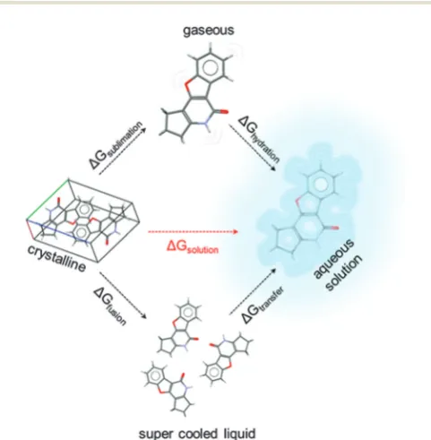
Two common approaches to the calculation of the Gibbs free energy of solution utilise a thermodynamic cycle approach. A first approach calculates the free energy of solution by addition of the free energy of sublimation (taking the molecule in the crystalline phase and subliming it into the gaseous phase) and free energy of solvation (taking the molecule in its gaseous phase and solvating it into aqueous solution). An example of this approach is shown in Section 5 of this review, and other examples are also cited within the literature.14,18,19A second approach involves calculation of the free energy of solution by addition of the free energy of fusion (taking a molecule from the crystalline state to a hypothetical supercooled liquid) and the free energy of transfer (transfer from a supercooled liquid into aqueous solution). This method is widely cited within the literature, and common GSE methods are also derived from this approach.5 Both thermodynamic cycle approaches are depicted in Fig. 1.

The solid state is an important consideration for the initial crystalline phase calculated within thermodynamic cycle approaches. Lattice minimisation calculations and periodic DFT provide excellent tools for modelling these systems. Recent advances in these methods show promise for improving predictions, these include updated codes and improved dispersion corrections in periodic DFT.20,21

Complete polymorphic screening and prediction still eludes our capabilities and hence hampers our ability to predict solubility from purely first principles.

A further consideration is that of the standard states used in the diﬀerent physical states. Typically sublimation data is reported in a 1 atmosphere standard state. Solvation is typically quoted in the Ben-Naim standard state of 1 mol L1with a fixed centre of mass. The diﬀerence between the two standard states is a constant 1.89 kcal mol1 (7.91 kJ mol1), calculated as DGatm - mol L1 = RTln(24.46), where 24.46 is the molar volume at ambient conditions.

The free energy of solution can be calculated directly by the following formula:

DGsolution ¼ RTlnðS0VmÞ

logðS0VmÞ ¼

DGsolution 2:303RT

(3)

whereS0is the intrinsic solubilityVmis the crystalline molar volume, R is the gas constant and T is the temperature in Kelvin (K).

A convenient formula19allows the solution free energy to be calculated using the native standard states, and removes the dependence on the crystalline molar volume:

S0¼

p0

RTexp

DG1 atm

sub þDG1 mol L 1

solv

RT

!

(4)

2. Informatics – ‘Smart’ machines in

solubility prediction

Informatics is the science of information processing, storage, and data mining. There are many applications and methodol-ogies available for this type of task. Commonly used methods in chemistry are QSAR/QSPR models which are built from known data. These models correlate structural features of molecules with physical properties of interest. A major supposition of QSPR is that molecules similar in structure will have similar physical properties, and for QSAR models, perhaps chemical or biological similarities. Therefore it is possible to train a model defining a specific relationship between structure and property/ activity on a training dataset, and apply it to similar molecules to predict their properties and activities. For this reason, QSAR/ QSPR models are not broadly applicable (i.e., they cannot be applied to molecules diﬀering considerably from the training set). While QSPR was once dominated by multiple linear regression, nowadays machine learning represents the state of the art. Both regression and machine learning protocols can identify these structure–property relationships by correlating structural features with experimentally determined physical data. A brief introduction to some of these methods is provided below, and for a more detailed account, see ‘‘An Introduction to Cheminformatics’’22,23 and references therein. Initially, one must represent a molecule in a machine readable format to enable the calculation of molecular descriptors. Two of the most common methods for doing this are the Simplified

Fig. 1 Calculating the Gibbs free energy of solution is often achieved

through the utilisation of thermodynamic cycles. Two routes are depicted here. The first route is shown at the top of the diagram, whereby a molecule is taken in its crystalline form and sublimed, and then hydrated. The addition of the Gibbs free energy terms of these processes gives the free energy of solution. The second thermodynamic cycle is represented at the bottom of the diagram, whereby the molecule is taken in its crystalline form and undergoes fusion into a hypothetical supercooled liquid, and then is transferred into aqueous solution. The addition of the free energy terms for these two processes also gives the Gibbs free energy of solution.

[image:3.595.48.289.365.611.2]

(4)

Molecular Input Line Entry System (SMILES)24and the IUPAC International Chemical Identifier (InChI).25

2.1 Molecular descriptors

Descriptors represent physical, chemical, topological or ener-getic features of chemical structures, and can vary greatly in form and derivation. In general, a descriptor is a vector of single numerical values (features), each encoding specific information about an individual molecule.22This information can be a simple number, such as the molecular weight or the count of a specific atom type, or they can be a prediction of corresponding experimental quantities, such as the octanol– water partition coefficient (usually expressed as logP). Alterna-tively, they can also be derived from semi-empirical or quantum chemistry. Clearly the cost of calculating different descriptors can vary dramatically. It is often the case that descriptors offering higher levels of refinement, and therefore more useful molecular discrimination, incur a higher computational cost.22 There are many different molecular descriptors and numerous pieces of software to calculate them.22

2.2 Methods

2.2.1 Regression.Regression analysis is a fundamental tool in informatics. Simple linear regression expresses a relationship between a scalar dependent variableYand a single explanatory independent variable X. Multiple Linear Regression (MLR) extends this to allow for multiple dependent yi variables or explanatory independent variablesxi, expressed as;

y¼X

j

i

aixi (5)

These methods have seen widespread use in many fields.26 A disadvantage of MLR is the apparent ease of over-fitting. It is suggested that a useful rule of thumb is that the number of data points should be in excess of five times the number of expla-natory variables (Fig. 2).22,23

2.2.2 Random forest. Random Forest (RF), is a learning method based on decision trees. These are stacked sets of binary separators following a tree like graph structure. RF uses a ‘forest’ of these decision trees, making use of ‘‘the wisdom of crowds’’; hence, it is considered an ensemble learning method. RF can be used for classification or regression. For application to classification problems, the binary splitting is based upon the Gini index, which is a calculation of the maximal discrimi-nation of the data points. For regression, splitting is generally based on a minimisation of the root mean squared error (RMSE). The initial node is known as the root node, with subsequent nodes being called branch nodes. The final nodes are referred to as leaf nodes and contain molecules with similar predictions of the property or activity (Fig. 2).14,23

2.2.3 Support vector machines. Another commonly used machine learning method is that of Support Vector Machines (SVM). SVM supports both regression and classification tasks, and is capable of handling multiple continuous and categorical variables. Methods for handling classification tasks are based on typically non-linear kernel functions. These kernel functions allow the transformation of data points into a higher dimensional feature space (Fig. 2).

SVM training algorithms are built up of binary categorised data, whereby a particular data point belongs to one of two categories. Thus, the test set data is also categorised, producing a clear separation, which should be as wide as possible, in the feature space. Alternatively, in the case of regression, the surface behaves analogously to a regression line, providing a maximal explanation of the data within the bounds of an acceptable error margin whilst attempting to remain relatively flat to avoid overfitting.22,23

2.2.4 Networks. Artificial Neural Networks (ANNs) and deep learning architectures are another common form of machine learning method in chemistry. These are models conceptually based on the brain’s neuron network (although a great simplifica-tion). ANNs contain an input layer which receives the molecular information, an output layer which provides the prediction to the

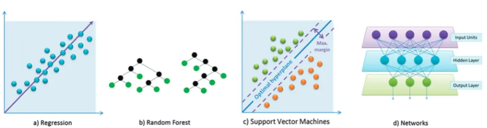
Fig. 2 Machine learning methods; (a) regression analysis aims to describe how the typical value of the dependent variable changes as the independent

variables are changed. The regression function (purple arrow) characterises variation; (b) decision trees consisting of a binary separation at the nodes, leading to predictions or classifications at the leaf nodes (green circles); (c) an example of SVM separating data into distinct categories by an optimal hyperplane, which should have optimal margins either side for a clear distinction in data categorisation; (d) a typical network consists of layers of nodes. All nodes have connections with all other nodes in adjacent layers. The input units (top) do not count as a layer of nodes, as they do not carry out any typical arithmetic operations. A typical arithmetic operation is the generation of a net signal and transformation by a transfer function into an output signal. The input units distribute input values to all of the neurons in the layer below. The connections between nodes each have a diﬀerent weight, representing diﬀerent descriptors used in machine learning.

[image:4.595.53.545.504.633.2]

(5)

user, and between these at least one hidden layer which is trained using data to link the neurons of the input layer and output layer in a suitable fashion for the problem at hand. The training generally involves weighting specific paths between the neurons.7,8,13 _{Deep learning architectures aim to enhance} the learning capabilities of machine learning methods such as ANNs. Deep learning algorithms attempt to abstract data on a high level through model architectures comprising multiple non-linear transformations. In the case of ANNs, enhanced data abstraction can be achieved through the addition of hidden layers, capturing the interaction of many factors which contribute to the observed data.

2.3 The General Solubility Equation (GSE)

GSE (as briefly mentioned in the introduction) is a QSPR model based on the melting point and the octanol–water partition coefficient logPof a chemical substance, used to predict the aqueous solubility of non-ionisable compounds,28and acts as a useful guide for ionisable compounds using lipophilicity (logD) at the pH of the aqueous buffer employed. The equation states that;

logS= 0.5–0.01(m.p.1_{C – 25)}_log_P ₍₆₎

Or in terms of logD;

logSpH(x)= 0.5–0.01(m.p.1C – 25)logDpH(x) (7)

GSE is a simple QSPR model, with powerful predictive ability (coeﬃcient of determination (r2) = 0.96 and root mean squared error (RMSE) = 0.53 logSunits for a data set of 1026 organic molecules29), and the simplicity of the model means it has found wide application in the pharmaceutical industry. How-ever, the reliance of the GSE on experimentally determined descriptors limits its applicability, and datasets sparsely popu-lated at their limits can lead to overestimation of the model’s predictive power.30

Ali et al.30 have revisited the GSE and have attempted to relieve the reliance of the GSE on the experimentally deter-mined melting point by replacing it with a descriptor that describes the topological polar surface area (TPSA). They demonstrate the eﬀects of inflated predictive power of the GSE by using a subset of an initial dataset, which reduced the overall predictive power of the GSE by approximately 6.4%. TPSA was included in a revised model to account for the fact that 88.5% of poorly performing compounds contained polari-sable groups. The pure GSE model employed provided r2 = 0.818, and the TPSA replacement of melting point model providedr2 = 0.813, showing a comparable eﬀectiveness. The number of compounds containing polarisable groups with logS predicted within 1 log unit of experimentally determined values was also higher for the revised TPSA model (83.2% TPSA; 79.6% GSE). A final model combining melting point, logPand TPSA was also tested, and was found to have a better predictive power than both of the previously employed models (r2= 0.869) with 90.8% of compounds containing polarisable groups pre-dicted within1 log unit of experimentally determined values.

The work of Aliet al.30highlights the importance of reliable descriptors in improving the overall performance of QSPR models, particularly when polar or polarisable functionality is included in test sets, and when experimentally determined values are required. As such, experimentally determined values may be best suited only for comparative analysis of predictive models to experimental data as a measure of performance in many cases.

2.4 Other cheminformatics applications

A recent approach to predict solubility proposed by McDonagh et al.14applied three models, exploiting both cheminformatics descriptors and theoretically derived thermodynamic properties. The initial models use theoretical chemistry and QSPR models alone, with further development combining the two approaches into a unified QSPR model. The developed models aim to calculate solubilities in agreement with experiment and in a reasonable time period. It was found that quantitatively accurate solvation free energies are unobtainable from the specific simple theoretical chemistry approach applied. The authors suggest that QSPR models are the most eﬀective method, when both time and accuracy are considered. The machine learning methods employed, which use a modest number of cheminformatics descriptors, predict solubility values comparable to those obtained with currently available commercial software.‡Notably, only a small improvement in accuracy was found on combining the two approaches. This suggests that the cheminformatics descriptors and the theoretically derived quantities are not very complementary, but duplicate much of the same information.14

Another recent approach, by Lusci et al.,27 applies deep learning to the solubility prediction problem. The deep learning method is based on recursive neural networks adapted for undirected graph representations of molecules. The method produces good predictions of solubility on a number of standard datasets in the field.27

A further example of a cheminformatics approach is demon-strated by Shayanfaret al.31who apply a simple QSPR model to the prediction of aqueous solubility of drugs, validated by cross-validation. A training set of 220 drug-like molecules was used to build a model with MLR. Six descriptors (solute, melting point, experimental logP, calculated Abraham solvation parameters, calculated ClogP values and calculated melting points) were regressed against experimental aqueous solubility from the literature to develop a three-variable model, calculating aqueous solubility from Abraham solvation parameters,ClogP and melting points. The three variable model was then tested with cross validation, and a final two-variable model was developed with the excess molar fraction of the compoundEandClogP. The two variables used gave anR2_{value of 0.934 and a standard error} estimatesof 0.893. The proposed model was compared to a GSE model and a linear/solvation/energy relationship (LSER) model. Correlations between each model’s computationally determined

‡A recent machine learning method and dataset proposed by some of the authors is available from the Mitchell group web server: http://chemistry.st-andrews.ac.uk/staﬀ/jbom/group/Informatics_Solubility.html

(6)

values of aqueous solubility with corresponding experimental values gave anR2= 0.62 for GSE,R2= 0.57 for LSER andR2= 0.66 for the proposed MLR method.

Recent work has also suggested that, contrary to popular arguments, the quality of the experimental data available is not the limiting factor for the predictive accuracy of solubility predictions obtained from cheminformatics models.32 This work may suggest that inherent limitations within the models are responsible for the largest part predictive errors.

3. Implicit solvation – an isotropic field

as a solvent representation

Continuum solvation models consider solvent as a continuous isotropic medium. An underlying assumption of implicit solvation models is that explicit solvent molecules may be removed from the model, provided that the continuous medium replacing them suﬃciently represents equivalent properties.

A simplification of continuum models can be thought of in terms of a Hamiltonian as;

Hˆtot_(r

M) =HˆM(rM) +HˆMS(rM) (8)

whereMrefers to a single solute molecule,Srefers to the solvent, and r refers to position. Solvent coordinates do not appear within the Hamiltonian term, exemplifying the representation of solute in a continuum, rather than as definite atoms, as with explicit models.HˆMS_{is a sum of diﬀerent interaction operators,} which can be expressed in terms of solvent response functions, indicated byQx(

-r0,-r0), where-rindicates a position vector, andx represents a contributing interaction. More in-depth discussions are available in textbooks specific to computational chemistry, such as that by Cramer,3_{and reviews by Tomasi}_{et al.}15

In a standard continuum model, generally represented by Polarisable Continuum Models (PCM), solute–solvent interaction energies can be represented by a number ofQxoperators. The free energy ofMis therefore described by an expression of five terms;

G(M) =Gcav+Gel+Gdis+Grep+Gtm (9)

with the order of terms corresponding to the best performing order of the ‘charging processes’, integration processes coupling a distribution function with a potential function. The terms are the free energy of cavitation, electrostatic energy, dispersion energy, repulsion energy and thermal fluctuation, respectively.

3.1 Continuum models for electrostatic interactions

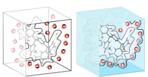
PCM models are advantageous in that they can represent a statistically averaged (continuum) solvent so that meaningful results can be acquired within a single calculation. PCM models have been particularly useful in modelling reactivity and spectroscopy of various solvents with diﬀerent polarities.33 In a solvent–solute system where atom Q (solute) has a positive charge, solvent water molecules will preferentially orientate their negative dipoles towards the solute’s positive charge (Fig. 3, left). For a single water molecule, there is only a slight preference in orientation, which is smaller than that of

its average thermal fluctuations. Therefore, this effect is averaged over the long range of electrostatic interactions of water in the bulk (Fig. 3, right). For an isotropic solvent with random thermal motion, the average electric field is zero at any given point. However, introduction of a solute gives a net change in orientation, introducing an overall change in electric field, known as the ‘reaction field’.

Accounting for the reaction field increases the solute’s polarity proportionally to the solute polarisability, and the strength of the external electric field. This causes an increase in the dipole moment of Q, consequently polarising and increasing the change in orientation of the solvent to oppose the dipole moment ofQ.3

There are energy costs associated with both the orientation and polarisation of the solvent, and the dipole moment ofQ. As solvent molecules oppose the dipole moment ofQ, they interact unfavourably with the reaction field. They also lose configurational freedom, with an associated free-energy cost. In a continuum model, the charge distribution of a solvent is represented as a continuous electric field, statistically averaged over all degrees of freedom at thermodynamic equilibrium. The electric field at any given point is the gradient of the electrostatic potential. The work required to create the charge distribution is determined from the interaction of solute charge densityrwith the electrostatic potential

ffrom;

G¼1

2 ð

rðrÞfðrÞdr (10)

The polarisation component of G, which we callGP, is the diﬀerence between charging the system in gas and solution phases; thus only the electrostatic potentials in both gas and solution phases are needed to calculateGP.

PCM methods are generally applied through two models: the Poisson–Boltzmann (PB) model, and the Generalised Born (GB) model. Both models are advantageous for different systems, and the accuracy of either model is mostly dependent upon the suitability of the cavity type used to surround the solute molecule within an ideal solvent system.

3.1.1 The Poisson–Boltzmann (PB) model. The Poisson equation (eqn (11)) combines the terms for electrostatic potential and the differential form of Gauss’s law to define the electrostatic

Fig. 3 (left) Water molecules reorient themselves to preferentially point

the negative end of their dipole towards the positive solute charge (+Q). (right) The system is modelled with a continuous polarisable field. Polari-sability is represented by the bulk dielectric constant,e.

[image:6.595.311.546.50.163.2]

(7)

potentialfas a function of the dielectric constanteand charge density r. When a surrounding dielectric medium responds linearly to an embedded charge, Poisson’s equation states that;

r2_f_ð_r_{Þ ¼}4prðrÞ

e (11)

Continuum solvation models represent the charge distribution on the basis of two separate areas: inside (solute) and outside (solvent) of a cavity (Fig. 4). For this case, the Poisson equation states;

re(r)rf(r) =4pr(r) (12)

The Poisson equation as expressed above is valid only for systems under non-ionic conditions. In a real solution, dissolving a solute produces mobile electrolytes. This eﬀect is accounted for by an expansion of the Poisson equation, known as the Poisson– Boltzmann (PB) equation;

reðrÞ rfðrÞ eðrÞlðrÞ8pq 2_I

ekBT

kBT

q sinh

qfðrÞ kBT

¼ 4prðrÞ

(13)

whereqgives the magnitude of electrolyte ionic charge,lis a function equal to 0 in areas inaccessible to electrolyte ions and 1 for accessible areas, and I indicates the ionic strength of the electrolyte system.

PB equations are best used to calculate the electrostatic potential of systems where the cavitation of solute is near-spherical or ellipsoidal (ideal cavitation), as the convergence of the predicted electrostatic component of the solvation free energyDGEis computationally expensive and often inaccurate. Thus, derivations applying approximations of the Poisson equation are often used in continuum models,33 the most common of which are Self-Consistent Reaction Field (SCRF) models, such as the Onsager model.34

A further limitation of PB based models is the definition of cavitation. A number of variational SCRF models have been proposed in order to optimise cavitation parameters, most commonly using tessellation (tiling) of the cavity surface to simplify and reduce iterations of the PB equation.33

3.1.2 The Generalised Born (GB) model. For systems in which ideal cavitation is not accurate, arbitrary cavitation can be applied. Arbitrary cavitation refers to the construction of a cavity around the solute similar to the shape represented by space-filling models generated from the overlap of atomic spheres at volumes representing van der Waals (vdW) radii. An alternative method to SCRF models involves an approximation of

the Poisson equation that can be analytically solved, known as the Generalised Born (GB) approach.

A conducting sphere with charge q can be considered representative of a monatomic ion. If the surface of the sphere is assumed to be entirely smooth, the charge distribution around it will be uniform, and the charge density at any point is given by;

rðsÞ ¼ q

4pa2 (14)

wheresis a point on the sphere’s surface, andais the spherical radius. Integrating over the entire outside surface and adding a term for the electrostatic potential, the energy termG, with |r| =a, becomes;

G¼ 1

2

ð _q

4pa2

q

ea

ds¼ q 2

2ea (15)

The Born equation for the polarisation of a monatomic ion is calculated from the diﬀerence in the required work in the gas and solution phases applied to eqn (8);

GP¼

1

2 1

1 e

q2

a (16)

The GB method extends the Born equation to polyatomic molecules to express polarisation energy as;

GP¼

1

2 1

1 e _Xatoms

k;k0

qkqk0g_kk0 (17)

wherekandk0_{run over all atoms, each with a partial charge}_q.

The determination of suitable parameters forgfor polyatomic systems involves a radial integration of the chargeqto deter-mine the interaction of atomkwith the surrounding medium.g

has units of reciprocal length, thus representing an inverse Coulomb integral.gis given a suitable functional form in order to approximate the PB equation, and has a limiting behaviour, becoming closer to the exact reciprocal length r1 at large interatomic distances.

3.2 Continuum models for non-electrostatic interactions

Similarly to the electrostatic components of solvation free energy, non-electrostatic contributions to the solvation free energy are not experimentally measurable. The solubility of experimental systems may be more susceptible to some eﬀects than others. Various neutral model systems have been devel-oped in accordance with this.

3.2.1 Specific component models. Pierotti35 developed a model formula, based on scaled particle theory, for the calcula-tion of cavitacalcula-tion free energy through the observacalcula-tion of the solvation energy for noble gases. Scaled particle theory is a statistical-mechanical theory of fluids derived from exact radial distribution functions, to give an expression for the work required to place a spherical particle into a fluid of spherical particles. Noble gas atoms do not exhibit permanent electrical moments, thus their transfer into solution is considered to be the most analogous example of perfect cavitation.

Fig. 4 The PCM cavity of allopurinol. (left) The solvent accessible surface

of allopurinol from a PCM calculation. (middle) The reaction field evalua-tion points. (right) Surface polarisaevalua-tion as a result of reacevalua-tion field.

[image:7.595.50.285.49.114.2]

(8)

The experimental data from Pierotti’s work has been com-plemented by simulation data,36including free energy of formation data of molecular-sized cavities in 12 common solvents obtained from free energy perturbation simulations. Pierotti’s formula has since been expanded for molecular cavities by Colominaset al.37

A further, specific contributing factor to solvation free energy is dispersion. A somewhat simplistic explanation of dispersion is as follows. The average electron cloud of an atom is spherically symmetrical, but at any instantaneous time point there may be a polarisation of charge causing an instantaneous dipole moment. This dipole moment interacts with neighbouring atoms, inducing a second instantaneous dipole, and so on, and an interaction occurs between these. The in-phase correlation of instantaneous and induced dipoles mean the overall interaction energy does not average to zero over time.3The average interaction energy falls oﬀ (largely) proportionally tor6(whereris the distance between interacting particles). The multipole expansion of the dispersion interaction is written;

VðrÞ ¼ C6

r6

C8

r8

C10

r10 (18)

whereC6,C8andC10are dispersion coeﬃcients dependent on the atomic species. This is normally evaluated as a sum over all pairs of atoms in diﬀerent interacting molecules.

3.2.2 Atomic surface tensions. Another approach for the evaluation of the non-electrostatic components of solvation free energy assumes the non-electrostatic component to be atom or group specific, and proportional to atomic surface area. A recent review by Wang et al.38 _{(2009) considers four QSPR aqueous} solubility models developed on the principle of weighted atom type counts and Solvent Accessible Surface Areas (SASA). They note that models considering SASA are often developed with small test-sets, and are therefore, in common with QSAR/QSPR models, poor performers for test molecules dissimilar to the original training set. The authors found that SASA descriptors did not enhance model performance any further than weighted atom type counts. This suggests the influences upon the non-electrostatic components of solvation free energy may be more complex than simple surface area considerations.

A further notable feature of continuum models based on surface tension is the neglect of any other contribution; that is, the development of these models assumes surface area as the sole determinant of solvation free energy, and that electrostatic components are implicit within the calculation parameters used.33

3.3 The current state of continuum models

There are a large number of available continuum solvent models, all with relative merits and shortcomings. The following is a brief description of those most commonly applied.

Integral Equation Formalism PCM (IEFPCM) is the current version of PCM applied in common quantum chemistry packages. IEFPCM is a reformulation of dielectric PCM (DPCM) in terms of the integral equation formalism. One of the biggest challenges to PCM methods is that they are all derived assuming the solute charge density is entirely encapsulated in the cavity.

This is often not the case, as the electron distributions often extend beyond the cavity. IEFPCM has been shown to cope well with this eﬀect when compared to other PCM based methods.33 A further variation of PCM is the conductor-like polarisable continuum model (CPCM), which is often considered one of the most successful solvation models.39_{The conductor-like screening} model/conductor-like screening model for real solvents (COSMO/ COSMO-RS)40 is a variation on Poisson–Boltzmann PCM and CPCM. In COSMO the dielectric permittivity (e) is set to infinity (e = N). This defines the solvent as a conductor, which is suggested as a more realistic approximation for strong dielectric media such as water, with the first version of COSMO40having values of the dielectric constant with a relative error of less than

1 2e

1_{. COSMO has been shown to be a reliable and readily} available method for calculations on the liquid and solution phases. The use of a boundary condition for the calculation of total potential in place of a traditional dielectric boundary con-dition for the electric field found values within 10% of the exact results obtained from dielectric boundary condition methods.41 COSMO-RS extends the COSMO code to also define the ability of the solvent to screen the surface charge on the cavity of the solute. Parametrisation of COSMO and COSMO-RS performed by the software developers tested 217 small to medium neutral molecules, spanning a vast functionality of H, C, N, O and Cl. An overall accuracy of 0.4 (rms) kcal mol1for chemical potential differences was achieved.41

A recent addition is the solvation model based on density (SMD). This model applies the IEFPCM protocol, solving the non-homogeneous Poisson equation using a set of optimised atomic Coulomb radii. The non-electrostatic contributions are calculated on the basis of a parameterised function which includes terms for atomic and molecular surface tensions as well as the solvent accessible surface area.42

A recent investigation of gas to solution phase standard state Gibbs free energies of solution compares energies obtained for six combustion gas flue compounds at the G4 level of theory using IEFPCM, CPCM and SMD implicit solvent models for 178 organic solvents. It is found that IEFPCM and CPCM produce similarDGSvalues for all six flue compounds, with maximum absolute intra-solvent deviations of o1.6 kJ mol1. Intra-solvent deviations between the IEFPCM and SMD models up to 45.5 kJ mol1 were observed. IEFPCM and CPCM also showed strong correlation between calculated solvent e and DGSfor all solvents, whereas SMD showed a much more varied relationship.43

4. Explicit solvation models

Explicit solvation models are the primary choice of solubility models where solvent-specific eﬀects are considered. The explicit treatment of water should, in principle, provide the most descriptive and realistic model for the investigation of solvation,44however it intrinsically requires a large number of degrees of freedom and thus is associated with a phase space of high dimensionality. This requires statistical averaging over the entire phase space, particularly

(9)

when extracting specific underlying physical behaviour, such as thermodynamic properties.

Statistical thermodynamics relates all observable thermo-dynamic properties to the partition function,Q. The partition function is summarised as;

Q¼

ðð e

Eðq;pÞ

kBT _d_q_d_p ₍₁₉₎

whereQis the classical formulation integrated over all phase space of all spatialqand momentumpcoordinates.

Explicit models consider solvation in terms of free energy calculations, with diﬀerent models for water available, as dis-cussed below.

4.1 Free Energy Calculations – Monte Carlo (MC) and Molecular Dynamics (MD) simulations

Free energy considerations are distinctly different for intramolecular and intermolecular degrees of freedom. For intramolecular components, free energy contributions rely on vibrational and librational motions on an intramolecular energy surface.45For well-defined energy-minima, the free energy is easily accessible from the partition function (eqn (19)) from vibrational frequencies treated with the harmonic approximation. The harmonic approxi-mation estimates the nuclear potential of a molecular system in its equilibrium geometry at a potential energy surface minimum in terms of normal vibrational modes, each governed by a 1D harmonic potential. Anharmonic effects are accounted for with MC or MD simulations for the calculation of entropy on the intramolecular energy surface.45Due to diffusion, the particles of a solution system do not exhibit motion definable by harmonic approximations. Thus, conventional MC and MD methods do not involve the direct determination ofQ, and exhibit an extremely slow convergence for densities of typical chemical systems, due to the exponential depen-dence of the Boltzmann factor on the occupation of available energy levels at a given temperature.

4.1.1 Free Energy Perturbation (FEP) methods.Free Energy Perturbation (FEP) methods were first introduced by Zwanzig46 in 1954, who related the thermodynamics of two diﬀerent systems, in order to evaluate diﬀerences in intermolecular potentials. Zwanzig notes that at high temperatures, the forces of repulsion between molecules determine the equation of state of a gas, and that at lower temperatures the equation of state should be determinable by considering forces of attraction as perturbations on the forces of repulsion. The energy change from state A to state B is calculated by;

DGðA!BÞ ¼GBGA

¼ kBTln exp

EBEA

kBT

A

(20)

whereTis temperature, and the triangular brackets indicate an average over the simulation runs for A. A normal simulation run for A coincides with a new energy state of B on each optimisation run. The energy diﬀerence between A and B is either between the atoms in each state, or in an isomeric diﬀerence, for example A may be thecis-isomer of a structure,

and B thetrans-isomer, with A and B in different energy states due to different intra- and/or intermolecular interaction. For isomeric differences, the free energy map is calculated along reaction coordinates. The convergence of FEP calculations is only reliable for a small difference between A and B, thus traditional perturbation theory only holds true for systems which remain similar upon dissolution.

More recent derivations of Zwanzig’s model allow the division of perturbations into smaller calculations, allowing parallelisation. These models involve breaking the reaction pathway down into a series of intermediate transition state steps, allowing better con-vergence between the initial and final structures investigated.47 However, FEP calculations remain one of the most computationally expensive methods for calculating free energy diﬀerences.

An example of this is shown by Lu¨der et al.48 who have investigated the eﬀectiveness of FEP methods for the calcula-tion of free energy of solvacalcula-tion in pure melts for 46 drug molecules. Simulations were performed in two stages, scaling down the Coulomb and Lennard-Jones (LJ) interactions inde-pendently. Results were interpreted under the assumption that the free energy of the vapour to liquid process DGvl can be calculated from the sum of the free energy term for cavitation DGcavand the energy associated with LJ interactions and half of the Coulomb interaction term. DGcav is obtained from hard-body theories. Interaction energies and molar volumes for each of the 64 drug molecules were compared for systems compris-ing 260 molecules. Deviations between systems were found to be an average of 2.9% for intermolecular interaction energy, and 1.4% for molar volume, suggesting the dataset selected would provide reliable results. Predicted and simulatedDGcavvalues are found to be systematically underestimated by approximately 15%. An overall average deviation of calculated DGvl values in comparison to experiment is1.8 kJ mol1, with reasonable errors expected in the range1 to 1 kJ mol1_{. This investigation suggests} that overall, FEP methods require more work at the theory level, particularly due to systematic errors that occur in phase space relationships between reference and perturbed systems.

An alternative approach to calculating the free energy diﬀerence from one state to another is to treat the change from A to B as a transformation, rather than to calculate free energies of independent structures, and calculate an energetic diﬀerence, as in traditional FEP methods.3

A recent application of this method, derived from FEP, has been demonstrated by Liu et al.49 for the calculation of the solubility of gases in ionic liquids. The Bennett acceptance ratio (BAR) method utilises the method of transferring between states instead of treating each state as an individual structure. The Coulomb and LJ terms are calculated separately. It is found that simulated solubilities are found in good agreement with Henry’s law constants. However, comparison to experimental data finds poorly soluble gases to have larger errors, with underestimated and overestimated gas solubilities found with similar calculation methods in complementary studies.

4.1.2 Enthalpy–entropy decomposition.A further offshoot of free energy calculations is the decomposition of the free energy term into enthalpic and entropic components. Entropy

(10)

and enthalpy complement free energy as they provide interpretive information to link molecular perturbations and thermodynamic changes. Two solutes may have similar hydration free energies (HFE), but may have solubilities dependent on distinct chemical functional groups.44 _{As both enthalpy and entropy are} mentally measurable, the difference between theory and experi-ment is ascertainable, and may be applied as benchmarks for force field optimisations,44and give insight into the mechanism of solvation. Levy and Gallicchio have reviewed a variety of different approaches to the thermodynamic decomposition of free energies.44 Wyczalkowski et al.50 recently proposed two new methods for the estimation of entropy and enthalpy decomposition of free energy calculations, evaluated for the solvation of N-methyl-acetamide (NMA). The methods investigated found thermo-dynamic contributions to be in disagreement with experimental data, highlighting the diﬃculty in obtaining decompositions comparable in quality to free energy estimates, with thermo-dynamic decomposition of computational Helmholtz free energies of solvation (DFat fixed volume) values yielding errors approximately two orders of magnitude larger than the initialDFvalues found. It is noted thatDFvalues are statistically reliable and can be used for quantitative comparison to experimental data. The calculation of entropic and enthalpic contributions is also extremely computation-ally demanding, as every temperature point of a simulation requires recalculation of the overall free energy.3The authors highlight that where calculation of free energies of solvation has advanced so that computational errors are on par with experimental ones, thermo-dynamic decomposition calculations suﬀer from statistical errors 10–100 times larger than free energy of solvation calculations.

A recent study by Ahmed and Sandler51uses the decomposition of free energies of hydration and self-solvation of low polarity nitrotoluenes to consider an array of thermodynamic terms and physiochemical properties. These include: solid-phase vapour pressures, solubilities, Henry’s law constants, hydration and self-solvation entropies, enthalpies, heat capacities and enthalpies of vaporisation or sublimation. Their study focuses on the temperature-dependence of various terms. Decomposition of hydration free energies into enthalpic and entropic contribu-tions is performed by a method utilising polynomial fitting of temperature-dependent self-solvation free energies (with respect to temperature). The use of fitting increases the sensitivity of derived values of hydration free energies. Self-solvation enthalpy (DHself) values and entropy (TDSself) values are calculated within approximately 2 kcal mol1of experimentally determined values.

4.2 Combined Quantum Mechanical/Molecular Mechanical Methodologies (QM/MM)

Explicit solvation models are often developed with respect to biological systems, due to the role of water in catalytic mechanisms, protein folding and protein–DNA recognition, to name but a few, which all require the specific detail of explicit water–substrate interactions to hold descriptive meaning. Of particular interest are combined QM/MM models, with QM describing electronic system changes (where precise system description is needed) and the rest of the system (where less precision is required) being

described by a MM force field.3Applications of QM/MM com-bined models are discussed in a recent review.52

The foundational concepts involve the partitioning of a desired system into two subsystems: the QM subsystem, con-taining a small number of atoms and described by QM, with the remainder of the system described by a suitable MM force field. The Hamiltonian of the whole system is simply written;

H=HQM+HMM+HQM/MM (21)

whereHQM is a QM Hamiltonian,HMM is an empirical force field andHQM/MMdescribes interactions at the QM/MM inter-face. The energy of the system is also described as the sum of QM, MM and QM/MM contributions. This model is often referred to as a two-layered approach (Fig. 5, left). A derivative of this model involves adding a third ‘‘layer’’ as a continuum solvent representation around the MM region, and is known as a three-layered approach (Fig. 5, right).

Theoretically, any desired level of accuracy can be used within the QM region of the simulated system, within the scope of available methods. However, more accurate methods are susceptible to high computational cost. Thus, careful consid-eration is required by the user as to what level of accuracy is required, and at what cost. A succinct overview of diﬀerent available QM methods is provided by Friesner and Guallar52for QM/MM methods applied to enzymatic catalysis, with descrip-tions, advantages and disadvantages of respective QM methods available in textbooks such as the one by Cramer.3

A primary consideration when selecting a QM/MM method is the interactions at the QM/MM interface. Two aspects must be considered; (i) the presence of covalent bonds across the interface – a particular concern for large (e.g., biomolecular) molecules, (ii) the influence of the MM solvent region on the QM region – electrostatic and van der Waals interaction terms must be included.

In order to treat covalent bonds at the interface, it is possible to introduce ‘‘link atoms’’. Link atoms are QM hydrogen atoms that fill free valencies of QM atoms connected to MM atoms. A disadvantage of this method is the debate about inclusion of

Fig. 5 (left) Two-layered approach to the QM/MM method. The solute

molecule and a few water molecules are treated with QM (centre) and the rest of the solvent system is represented by MM up to a user-defined distance. (right) Three-layered approach – an additional layer surrounds the MM region and uses a continuum approach to describe the long range solvent in the bulk.

[image:10.595.307.550.525.652.2]

(11)

Coulombic interaction terms for the link atoms. Other methods developed in order to avoid the use of link atoms include the Local Self-Consistent Field (LSCF) method, which applies a mixture of hybrid and atomic orbitals to represent the QM system, and the ‘‘connection atom’’ method, where MM and QM interface atoms are described as QM methyl groups with a free sp3_valence.

A recent three-layered approach aiming to tackle the issues associated with the QM/MM interface and the interaction terms for MM solvent eﬀects has been proposed by Steindalet al.53 This approach is described as the fully polarisable QM/MM/PCM method (see Section 3 for a description of PCM), and is designed for the eﬀective inclusion of a medium in a QM calculation. Short range solvent electrostatic potentials are described by an atomistic model (QM/MM) whilst the long range potentials are described by a continuum. The method is implemented in combination with linear response techniques with a non-equilibrium formulation of environmental response. The authors find a faster convergence with respect to system size for QM/MM/PCM than for QM/MM methods. This approach allows for reduction of the MM part of the calculation with PCM, allowing less demanding calculations, and reduced sampling. However, three-layered approaches such as this often require much more user input and method manipulation, for example, considerations for MM/PCM interactions have to be considered in addition to QM/MM interactions, and so such methods are suited only to advanced users.

4.3 Explicit representations of water atoms

When solvent is represented explicitly, solvent molecules usually greatly outnumber solute molecules. Thus, in order for a model to be eﬃcient, it is advantageous to use the simplest possible solvent representation.44 Water is often considered the most useful solvent system, and thus is the solvent most widely used in explicit solvent models. The macroscopic properties are well established, yet the microscopic forces that determine water structure are not fully understood.

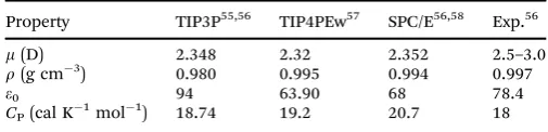
The treatment of water can be rigid or flexible. Rigid models often include a fictitious H–H bond to constrain bond angles in the water monomer.3Three of the most common rigid models for water are the TIP3P (transferable intermolecular potential 3P), SPC (simple point charge) and SPC/E (simple point charge extended) models, and their modified counterparts. These three models are effectively rigid pair potentials comprising LJ and Coulombic terms. However, the terms used differ in each model, and give rise to different calculated bulk properties for water.54_{Values for various properties of water obtained with} different rigid models of water are shown below, in Table 1.

MD calculations require the integration of Newton’s equations of motion for all atoms, which is achieved through the evaluation of all atomic forces at each time step. Non-bonded interactions, especially long-range electrostatic interactions, dominate computa-tionally, requiring extensive CPU time. In order to minimise this to an acceptable level, approximations are necessary. Boundaries are introduced into water models to restrain the system to a finite size, which almost always leads to artefacts in the obtainable data.54The most commonly utilised method for cost-effective solute computa-tions is the application of a spherical cut-off, limiting the number of pairwise interactions to those within a specified radius.54The use of cut-offs for non-bonded interactions can have undesirable effects. LJ interactions are susceptible to small energetic effects, and large pressure effects induced by cut-offs. Pressure scaling can be used to correct for pressure related cut-off effects, usually to the order of several hundred bar. Cut-off effects for systems with dipolar electrostatic interactions are more prominent, with cut-offs selected within the parameters of experimental radial distribu-tion funcdistribu-tions up toB1.0 nm. However, computer simulations have shown ordering within water up to B1.4 nm, so the full structure of water is not typically accounted for, resulting in a poor description of dielectric properties. A further, and the most promi-nent, effect of cut-offs occurs in systems with full charges, where accumulation of the charge occurs at the cut-off boundary.59

Spoelet al.59(1998) investigated the effectiveness of TIP3P, TIP4P, SPC, and SPC/E models in describing the density and energy, dynamic, dielectric and structural properties of water. All simulations and analyses were identical for each model investigated, allowing the evaluation of simulation methodology independent of the model. It was found that system size, cut-off length and reaction fields had comparable effects on the overall calculated structural properties of water.

System size effects are considered through the comparison of systems comprising a small (216) and a large (820) number of molecules. The average thermodynamic properties (r,Epot,T,P) are the same regardless of system size. Fluctuations in thermo-dynamic properties are known to be proportional to the square root of the system size, which is confirmed within the study. However, differences between large and small systems are observed, particularly for the dielectric constant, which is higher for all systems with a large number of molecules. The diffusion constant for large systems is also higher, attributed to periodic boundary conditions (PBC).

Cut-off effects are considered by the use of two different cut-off lengths (0.9 nm and 1.2 nm) for the large systems. It is found that density increases with an increased cut-off length, and energy decreases. There is no effect on dielectric behaviour. In all simulations density decreased by approximately 1 kJ mol1 on application of a reaction field. The self-diffusion constantD, and rotational correlation times were found to increase, indicating that the reaction field affects both the translational and rotational mobility of molecules.

[image:11.595.40.293.659.720.2]

Quantum chemical MD simulations of water are often developed with Density Functional Theory (DFT) methods, using either plane wave or atom-centred basis sets, to deter-mine the electronic structure and forces. These methods oﬀer

Table 1 Modelvs.experimental (exp.) values for bulk properties of water

under standard conditions (298 K; 1 bar), including dipolem, densityr, static dielectric constante0and heat capacityCp

Property TIP3P55,56 TIP4PEw57 SPC/E56,58 Exp.56

m(D) 2.348 2.32 2.352 2.5–3.0

r(g cm3) 0.980 0.995 0.994 0.997

e0 94 63.90 68 78.4

CP(cal K1mol1) 18.74 19.2 20.7 18

(12)

reasonable estimates of the structural and dynamic properties of water when compared to experimental measurements. However, problems exist in the description of electronic gradient corrections, and equilibrium pressure. The interatomic forces of early quantum simulations, including DFT based methods, were originally para-meterised with classical mechanics, leading to an unsatisfactory agreement between quantum and experimental results. DFT models also tend to calculate liquid structure with too much order, and underestimate equilibrium density. This is often attributed to the inability of local functionals to describe dispersion eﬀects.

A recent approach to water simulation has claimed to provide a model, called the electronically coarse-grained model, capable of accounting for the shortcomings of both existing classical and quantum models.60Joneset al.60(2013) base their method on the replacement of valence electrons of an atom with an embedded Quantum Drude oscillator (QDO). QDO treatment of water is based upon the TIP4P classical rigid model of water, with the three water atoms supplemented by a dummy atom with a negative charge, added along the+HOH bisector to create an additional interaction point. The QDO parameters aim to reproduce the isotropic parts of the dipole, polarisability, and the dispersion coefficient. The dispersion interaction is then adjusted by scaling, whilst preserving polarisability. The baseline unadjusted model produces a rea-listic, but over-structured liquid with a density that is too low by up to 20%, attributed to its underestimation of dispersion. Note also that the value of the enthalpy of vaporisation (at ambient pressure) Dhvap was found at 40 2 kJ mol1, close to the experimental value of 43.91 kJ mol1. Scaling the dispersion term results in an increased equilibrium density for increased dispersion. This induces a weakening effect on the H-bonding network of water, bringing the overall structure closer to agreement with benchmark data. However, the calculatedDhvap increases to 46 2 kJ mol1_{, which is 4% higher than the} experimental value. It is also found that the H-bond network is sensitive to changing polarisation at fixed dispersion, affirming the independent importance of both polarisation and disper-sion effects on an overall explicit model.

5. Eﬃcient hybrid models – statistical

mechanics

Within an aqueous solution phase, single snapshot images of structure are of limited use. Water is one of the few single component liquids for which there are highly competitive interactions at short range (hydrogen bonding), capable of damping the eﬀects of repulsion. For this reason, ensemble averaging is required to identify the most probable geometric configurations which most heavily contribute to the system’s interactions. This idea has already been introduced within explicit models of solvation using ensembles taking snapshots at specific time periods. However, the cost of calculating the many configurations accessible in a solution is enormous,

hence, in this section we focus on statistical mechanics meth-ods which enable a more eﬃcient calculation process.

5.1 Correlation functions

From a chemical point of view, a solution is a highly mobile system in which the dynamics are a vital contribution to the system’s properties and behaviour. Therefore, mathematically we wish to capture this. Attempting to quantify dynamics with static properties is not suﬃcient; we must therefore provide averages or probabilities of interactions occurring at given distances. For this reason a natural choice is to represent the solvent using Pair Correlation Functions (PCF), or equivalently Radial Distribution Functions (RDF). These functions allow us to determine a probabilistic structure of the solvent.

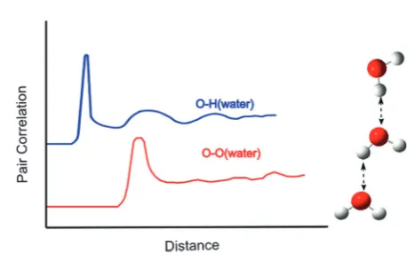
PCF can be interpreted as showing the probability against distance of there being an atom of interest at that distance from the atom under study. For example the first large blue peak in Fig. 6 would correspond to either a water H at a distance from an O atom under study or vice versa. These functions are experimentally determinable from scattering experiments. We would expect that the PCF/RDF would go to a constant value of 1 at large values of r (i.e. it would become isotropic, like a continuum model, as there are no solute interactions to perturb the system). However, at small values ofrwe would not expect this. At very small values (less than the van der Waals radii of the solute atoms) we expect zero as only one particle can occupy the space at a time. Just outside this distance we see sharp non-uniform behaviour as solvent in the space interacts favourably with the solute holding a more rigid form. This leads to troughs in the PCF/RDF just behind the peaks, thus deviating from the value of 1 for a uniform solvent (Fig. 6).

5.1.1 Computational use and determination of correlation functions.The starting point for the use and determination of these functions for solvation modelling in statistical mechanics is integral equation theory (IET). In this theory a molecule is fully described by a six-dimensional vector (three degrees of freedom relate to positionx,y,zand three degrees of freedom determine the orientationc,y,j). To refer to these two sets of variables collectively, we will use the following symbolsr= {x, y, z} and Y = {c,y, j}. These variables are conveniently incorporated into the fundamental 6D integral equation, the

Fig. 6 A schematic representation of PCF for liquid water; water oxygen –

water hydrogen (blue) and water oxygen – water oxygen (red).

[image:12.595.309.543.550.693.2]

(13)

Molecular Ornstein–Zernike equation (MOZ). This equation utilises PCF/RDF between the various constituents of the liquid, g(r1, r2, Y1, Y2). This simplifies for homogeneous solution to relative positions and orientation of the constitu-ents,g(r1r2,Y1Y2). This can most conveniently be written with reference to the total correlation functionh(r,Y).61

hij(r1r2,Y1Y2) =gij(r1r2,Y1Y2)1 (22)

We can simplify this equation by assuming spherical symmetry of molecules, hence removing consideration of orientational degrees of freedom by treating each water molecule as a hard sphere. We can now further separate the contributions to the total correlation function into direct and indirect components. To do this we must introduce the direct correlation functionc(r). We can now re-write the MOZ equation assuming spherical symmetry as follows:

h r1;2

¼c r1;2

þ ð

dr3c r1;3

rðr3Þh r2;3

(23)

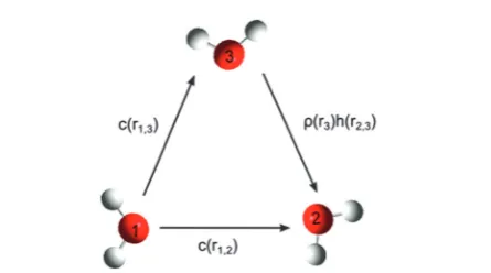
Two eﬀects contribute to the total correlation function (eqn (22)): (i) the direct correlation betweenr1andr2, and (ii) an indirect correlationviaa third body,r3. The indirect correlationvia r3is weighted by the density atr3, and thus allows the consideration of all possible positions of the third body (Fig. 7).61

To solve this equation,h(r) andc(r) need to be found. As we have only a single equation and two unknown functions,h(r) andc(r), another equation is required; a closure relation must be introduced. There are several such equations available from statistical mechanics. The exact closure relation is as follows:

g(r) = ebU(r)+h(r)c(r)+B(r))ebU(r)+T(r)+B(r) (24) wherebis equal to 1/kBTandU(r) is the interaction potential which is often of the following form:

UðrÞ ¼4e sab r

12

sab

r

6

þqaqb

r (25)

T(r) is known as the indirect correlation function as it is the diﬀerence between the total and direct correlation functions, and quantifies the indirect contribution. B(r) is the bridge function, which comes from graph theory – its exact form is not known. Several approximate closure relations exist; some will be discussed here, although others are available. Originally the HyperNetted-Chain (HNC) approximate closure was used:

h(r) = e(bU(r)+T(r))₁ ₍₂₆₎

This closure works in principle for charged systems but neglects the bridge function term completely, assuming it to be zero. This can lead to poor convergence due to uncontrolled growth in the argument of the exponent. An alternative is the Partially Linearised HyperNetted Chain (PLHNC). This closure linearises the HNC once a cut oﬀ value (C) is exceeded:62

L ¼ bUðrÞ þTðrÞ

hðrÞ ¼ e

bUðrÞþTðrÞ

ð Þ₁ _when_L_C

bUðrÞ þTðrÞ þeC_C₁ _when_L₄_C

( ₍₂₇₎

This improves the convergence of the equations and is now regularly used in many applications for a variety of systems.

Due to the spherical symmetry approximation, the MOZ can only be applied to simple solutions. Additionally, due to the high dimensionality of the full equation, before the spherical symmetry approximation was invoked, it was practically incomputable. For this reason a number of approximations have been developed which are collectively referred to as Reference Interaction Site Models (RISM).

5.2 3D-RISM: a hybrid solvation model

As we have seen, the explicit treatment of solvent is considered to be a necessary step in the understanding of solvent structure. However, this naturally carries high computational costs.3The alternative continuum treatment of solvents lacks the ability to account for the underlying physical theory; energy contribu-tions from solvation shell features are computable, but not transferable. Solvent structure features from the first and second solvation shells are lost in continuum models, and non-electrostatic energy terms are not described from first principles, thus are not transferable to more complex models.63 The 3D derivation of RISM (3D-RISM)64,65is a 3D molecular theory of solvation, applied through solvent distributions, rather than explicit solvent molecules, and conceives solvation structure and dynamics from the first principles of statistical mechanics.

3D-RISM is derived from a partial integration over the orientational degrees of freedom; this leaves a set of 3D integral equations (one equation per solvent site;Nsolvent). This method utilises solvent site – solute total correlation functions and direct correlation functions in the solution of the RISM equa-tions. The 3D-RISM equations take the following form:62

hðaÞ ¼ X

Nsolvent

x

ð

R3

cxðr1r2Þwx;aðj jr2Þdr2 (28)

here wx,a labels the solvent susceptibility function. This

func-tion models the bulk solvent mutual correlafunc-tions. For the example of water, this function models the intermolecular correlation between water oxygen and water hydrogen. This function can be calculated from the intramolecular solvent correlation function (osolventzg (r)), the radial site to site total

Fig. 7 Illustration of the contributions, both direct and indirect, to the

total correlation function.

[image:13.595.59.282.569.693.2]