Mixture models for distance sampling detection functions

Mixture Models for Distance Sampling

Detection Functions

David L. Miller*, Len Thomas

Centre for Research into Ecological and Environmental Modelling, and School of Mathematics and Statistics, University of St Andrews, St Andrews, Scotland, United Kingdom

*[email protected]

Abstract

We present a new class of models for the detection function in distance sampling surveys of wildlife populations, based on finite mixtures of simple parametric key functions such as the half-normal. The models share many of the features of the widely-used“key function plus series adjustment”(K+A) formulation: they are flexible, produce plausible shapes with a small number of parameters, allow incorporation of covariates in addition to distance and can be fitted using maximum likelihood. One important advantage over the K+A approach is that the mixtures are automatically monotonic non-increasing and non-negative, so con-strained optimization is not required to ensure distance sampling assumptions are hon-oured. We compare the mixture formulation to the K+A approach using simulations to evaluate its applicability in a wide set of challenging situations. We also re-analyze four pre-viously problematic real-world case studies. We find mixtures outperform K+A methods in many cases, particularly spiked line transect data (i.e., where detectability drops rapidly at small distances) and larger sample sizes. We recommend that current standard model se-lection methods for distance sampling detection functions are extended to include mixture models in the candidate set.

Introduction

Distance sampling [1,2] is a suite of methods for estimating the size or density of biological populations. There are two main variants: line and point transects. In both, an observer visits a randomly-located set of transect lines or points and records the distance,y, from the transect to each object of interest (i.e., animals or plants of the target species) that is detected within some truncation distancew(after which no observation is recorded; truncation may be chosen after the survey has taken place, see Buckland et al [1] for further discussion). Not all objects withinware assumed to be detected; instead the observed distances are used to estimate the pa-rameter vector,θ, of a detection function model,g(y;θ), which describes how the probability of detection declines with increasing distance. An assumption of the conventional method is that

g(0;θ) = 1. Given an estimate ofθ, it is straightforward to estimate population size or density (see below).

OPEN ACCESS

Citation:Miller DL, Thomas L (2015) Mixture Models for Distance Sampling Detection Functions. PLoS ONE 10(3): e0118726. doi:10.1371/journal. pone.0118726

Academic Editor:Thierry Boulinier, CEFE, UNITED STATES

Received:August 19, 2014

Accepted:January 15, 2015

Published:March 20, 2015

Copyright:© 2015 Miller, Thomas. This is an open access article distributed under the terms of the

Creative Commons Attribution License, which permits unrestricted use, distribution, and reproduction in any medium, provided the original author and source are credited.

Data Availability Statement:Data on long-finned pilot whales are available on request from the Marine Research Institute, Iceland (http://www.hafro.is). All other data files are available from Figshare (DOI:

http://dx.doi.org/10.6084/m9.figshare.1293041).

Funding:The authors received no specific funding for this work.

A key part of distance sampling, therefore, is specification of the detection function model. Buckland et al. (Chapter 2) [1] provide a set of criteria for judging the utility of candidate model classes. Detection function models should be:

1. flexible, so that they can take a wide variety of shapes;

2. efficient, in the sense that many plausible shapes can be represented using few parameters; 3. flat at zero distance (i.e.,g0(0;θ) = 0), indicating that objects in the immediate vicinity of the

observer are equally detectable; and,

4. monotonic non-increasing with increasing distance (i.e.,g0(y;θ)0 for 0<yw), as it is typically unrealistic for objects to become more detectable with increasing distance. The semiparametric“key function plus series adjustment”(K+A) modelling approach de-veloped by Buckland [3] has become by far the most popular in practice, partly due to its inclu-sion in the industry-standard distance sampling analysis software Distance [4] and the R [5] package mrds [6] (available on the Comprehensive R Archive Network, CRAN; http://cran.r-project.org/). However, as we demonstrate below, the approach has some drawbacks; in partic-ular, although it meets criteria 1–3, it does not necessarily meet the 4th. Our purpose in this ar-ticle is to propose an alternative class of models, based on mixtures, that meet all 4 criteria and to evaluate its utility.

The approach of Buckland [3] was extended by Marques and Buckland [7] to allow covari-ates in addition to distance to be included in the detection function, and, for maximum gener-ality, it is this K+A formulation that we describe here. The detection function is thus denotedg

(y,z;θ) wherezis an observation-specific vector of covariates; the formulation of Buckland [3] is simply a special case of this model where there are no additional covariates.

In Marques and Buckland [7], the detection function is modelled as a parametric key func-tionkand series expansionsof even functions (known asadjustment terms) with some param-etersθ.gis then written as:

gðy;z;θÞ ¼kðy;z;θÞf1þsðy;z;θÞg

kð0;z;θÞf1þsð0;z;θÞg;

wherekmay be a half-normal, hazard-rate or uniform function andsmay be zero (i.e., there are no adjustment terms), cosine, simple even polynomial or Hermite polynomial series (though note a uniform detection function may not include covariates). The denominator en-sures that detection function evaluates to 1 at zero distance (i.e.,g(0,z;θ) = 1). Model parame-ters are estimated using maximum likelihood. The recommended strategy for most situations is to choose a small set of key function and adjustment combinations, and for each combina-tion to choose the number of adjustment terms using forward seleccombina-tion, i.e., start with no ad-justment terms andfit an increasing number of terms, stopping when the Akaike Information Criterion (AIC) fails to decrease [4]. The combination with the lowest AIC is then selected as the best model. This strategy works well in practice in many cases: the key functions cover a range of realistic shapes for the detection function, so that often zero or one adjustments are sufficient to provide a goodfit to the data, resulting inflexible and yet efficient estimation.

The resulting detection functions are capable of being flat at zero distance and the key func-tions are non-increasing. However, adding adjustment terms can result in non-monotonic functions. Further, when both covariates and adjustments are included in the model the range of the resulting detection function may not be [0, 1]. When there are no additional covariates, one solution is to use constrained maximization, e.g. takingMequally spaced distances

i= 1,. . .,M−1. In Distance this constraint is implemented using the NLPQL routine [8] and in the R package mrds, the SOLNP algorithm [9] is used.

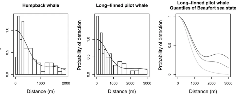
A constrained optimisation solution presents a number of problems. First, constrained max-imization is a more complex optmax-imization problem than unconstrained maxmax-imization; this means that in practice optimization algorithms may fail to find the constrained maximum. Sec-ond, constrained maximum likelihood estimates do not have the same appealing properties as their unconstrained relatives—for example the usual estimator of the standard error of the pa-rameters (square root of the inverse of the information matrix) can be biased. Third, con-straints can only be applied at a finite number of points (M= 10 is used in Distance andM= 20 in mrds by default), which can lead to the constraint points missing non-monotonic parts of the function. Though increasing the number of points is an option, this incurs additional computational cost. An example of constrained maximisation failing is shown in the left panel ofFig. 1. Finally, it is not clear how to implement the constraints in the case where there are ad-ditional covariates, particularly continuous covariates. One computationally expensive option would be to apply the constraints at every observed covariate combination (at present both Distance and mrds use unconstrained optimization when additional covariates are in the model). The central and right panels ofFig. 1from Pike et al. [10] show an example of covariate models fitted using unconstrained optimisation: a strongly non-monotonic function has been fitted for some covariate values. Detection probability estimates outside the range [0, 1] are sometimes encountered during maximization when models include covariates. Given the above issues, it seems appealing to use a formulation that guarantees monotonicity from the outset.

Mixture models have been applied in the capture-recapture literature [11–14]. The main utility of mixture models in capture-recapture is in better accounting for between-individual heterogeneity, which can cause severe bias if unmodelled [15]. Unmodelled heterogeneity is not generally considered an issue in distance sampling, provided that detection at zero distance is certain, heterogeneity is not extreme and a flexible detection function model is used ([2], Sec-tion 11.12). Mixture models come in two variaSec-tions: finite (consisting of discrete components) and continuous (infinitely many components, amounting to an integral with a weight func-tion); we consider only finite mixtures here (seeDiscussionfor further elaboration). Finite mix-ture models offer the potential for flexible modelling since the individual parts of the mixmix-ture model (themixture components) can be combined to obtain flexible detection functions, and provided each component is monotonic non-increasing, the resulting combination will also be monotonic non-increasing. In addition, mixture models are potentially well suited to deal with highly heterogeneous detection probabilities, where some part of the population is only observ-able at close distances while others are readily detected almost regardless of distance (for exam-ple bird species where males are more vocal than females). Such a situation results in a

“spiked”detection function with a long flat tail—Fig. 1shows relatively mild examples. In a mixture model, different parts of the sample could be represented by different components, providing a good fit to spiked data and an appealing conceptual explanation for the underlying data.

package, mmds [16] (Mixture Model Distance Sampling), implementing the methods is avail-able from CRAN.

Methods

Finite mixture model detection functions: Formulation

Denoting the detection function asg, we consider a sum ofJmixture componentsgj, scaled by some mixture proportionsϕj:

gðy;z;θ; Þ ¼X

J

j¼1

jgjðy;z;θjÞ;

wherePJj¼1j¼1. The distance is denotedy, theθjs are vectors of parameters for functiongj,

θis a vector of all of theθjs,fis aJ-vector (i.e., vector of lengthJ) of all of theϕjs, andzis a

K-vector of the associated covariates.

Although other monotonic functions such as hazard-rate could be chosen, and thegjs need not all have the same form, here we let thegjs be half-normal functions:

gðy;z;θ; Þ ¼X

J

j¼1

jexp y2

2sjðzÞ 2

!

:

Although each mixture component has a different scale, the covariates affect the scale pa-rameters in the same way (though other, more complex, models may be possible).

Covariates are included as in Marques and Buckland [7], by decomposing the scale parame-terσ(see also Marques et al. [17]). Usingito subscript each observation, our formulation for Fig 1. Two examples of detection functions that are not monotone, fitted using conventional key function plus adjustment methods in the software Distance.The left panel shows data from humpback whale: a half-normal detection function with cosine adjustments was selected by AIC [20] but even with constraints in place the detection function is non-monotonic, with a small secondary peak at approx. 1500m. The second and third panels show data and models fitted to long-finned pilot whale where a half-normal detection function was selected with cosine adjustments and Beaufort sea state as a covariate [10]. Due to the inclusion of covariates, no monotonicity constraints could be employed. The middle panel shows the detection function averaged over the covariate values and the right panel the marginal detection function for 25th, 50th and 75th quantiles of the Beaufort sea state covariate; non-monotonicity occurs at approx. 2500m.

the scale parameterσij, is

sij¼expðb0jþ

XK

k¼1 bkzikÞ;

wherezikis thekthcovariate for theithobservation. In this caseθwill contain theβ0js andβks. We can write the pdf of the observed distances conditional on the observed covariates as [2]:

fðyjz;θ; Þ ¼RwpðyÞgðy;z;θ; Þ 0 pðtÞgðt;z;θ; Þdt

:

whereπ(y) is the pdf of object distances (observed and unobserved). The likelihood can then be formed by taking product of these pdfs over thenobservations. The specific form of the like-lihood differs between line and point transects, because sampler geometry means that the form ofπ(y) is different for lines and points. For line transects, with random line placement, we ex-pect an equal number of objects at all distances from the line, and henceπ(y) = 1/w(wherewis again the truncation distance). The likelihood is then given by:

Lðθ; ;yjz1;. . .;znÞ ¼

Yn

i¼1

fðyijzi;θ; Þ

¼Yn

i¼1

gðyi;zi;θ; Þ

miðziÞ

¼Yn

i¼1 PJ

j¼1jgjðyi;zi;θjÞ

miðziÞ

whereμi(zi), theeffective strip width(for covariate combinationzi), is given by:

miðziÞ ¼

XJ

j¼1

j

Z w

0

gjðy;zi;θjÞdy: ð1Þ

For point transects, with random point placement, the expected number of objects increases with increasing distance from the point, and henceπ(y) = 2y/w2, giving

Lðθ; ;yjz1;. . .;znÞ ¼

Yn

i¼1

fðyijzi;θ; Þ

¼Y

n

i¼1

2pyigðyi;zi;θ; Þ

ni

¼Y

n

i¼1

2pyi

PJ

j¼1jgjðyi;zi;θjÞ

ni

whereνi, theeffective area of detection(for covariate combinationzi), is defined as:

ni¼2p

XJ

j¼1

j

Z w

0 ygj

ðy;zi;θjÞdy: ð2Þ

Akaike’s Information Criterion (AIC), and goodness-of-fit of fitted models can be assessed just as for K+A models using, for example quantile-quantile plots and Kolmogorov-Smironov tests (see Buckland et al. [2], Section 11.11).

In this article, we assume the distance data are in the form of“exact”object-transect dis-tances; alternatively, distances can be grouped into intervals, with pre-defined cutpoints (e.g., 0–10m, 10–20m, etc.), so that the data are the distance interval of each observation. In this case, a multinomial likelihood is obtained (see, e.g. Buckland et al. [1], Section 3.3.2). Also, in some cases (e.g., some aerial surveys), objects below a defined distance are not counted— so-called“left truncation”([1] Section 4.3.2). The likelihood is readily amended to account for this, by changing the lower limit of integration inequation (1)or (2).

Estimating population size

Population size can be estimated using the Horvitz-Thompson-like estimator [7]: ^

N ¼A

a

Xn

i¼1

1 ^

pi

ð3Þ

whereAis the area of the study region for which population size is being estimated,ais the size of the sampled area, andpiis the probability of theithobservation being detected given it is within the sampled area. For line transects,a= 2wLwhereLis the total line length, and

^

pi ¼

1

w

XJ

j¼1

^ j

Z w

0 gj

ðy;zi; ^θjÞdy:

For point transects,a=πw2kwherekis the number of points, and ^

pi ¼

2p

w2

XJ

j¼1

^ j

Z w

0 ygj

ðy;zi; ^θjÞdy:

A standard summary statistic is the average detection probability for an animal within the sam-pled area,P^a, which is given by:

^

Pa ¼n=N^:

Estimators for the variances ofN^ and^Paare given inS2 Text.

Examples

Simulated data. We wish to ensure that the class of models we propose can be applied to a wide variety of situations that may arise. Extensive simulations were therefore carried out to in-vestigate performance (in terms of the accuracy of estimation ofPa) when the true detection function model is not known to the estimation procedure. The average detection probability,

Pa, is related to the estimated abundance as seen above and is easily calculated as a simple sta-tistic to summarise and compare the fitted models.

Each simulation involved generating 200 replicate datasets from a specified detection func-tion model (assuming the entire study area was included within the surveyed transects, i.e.,A=

ainequation (3), and a truncation distance ofw= 1), fitting each dataset with a range of mix-ture and key series plus series adjustment (K+A) models, and in each case recording estimated parameter values and abundance from the model with the lowest AIC in each of: mixture mod-els, K+A modmod-els, and both combined. Mixture models with 1-, 2-, and 3-point half-normal components were fitted to the data along with two K+A models: half-normal plus cosine ad-justments and hazard rate plus simple polynomial adad-justments, both with monotonicity con-straints implemented as described above and with a maximum of 3 adjustments. Mixture models and K+A models were fitted using the R packages mmds (version 1.1) and Distance [19] (a simplified interface to mrds; version 0.6.1) respectively, both written by the authors.

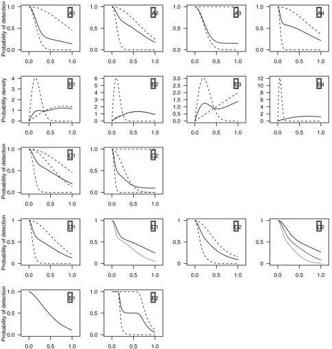
Fourteen different simulation scenarios were investigated, in five groups, as described below and illustrated inFig. 2, one line per group. True parameter values and summary statistics are given inS2 Appendix. For each scenario, a simulation was performed at each of five sample sizes (number of observations,n): 30 (low), 60 (recommended minimum for line transects [1]), 120 (adequate), 480 (large) and 960 (very large). We anticipated performance would depend upon sample size, because: the methods are likelihood-based and hence only asymptotically unbiased even if the correct model is fitted; the use of AIC to select model complexity meant that more flexible (and hence accurate) models could be expected to be selected given larger sample sizes. Mixture models are“parameter hungry”compared with K+A models, in the sense that each additional mixture component requires 2 extra parameters, while each addi-tional adjustment term requires only one and hence, given the use of AIC for model selection, the relative performance of the two approaches may change at different sample sizes.

Group A. Line transect with 2-point half-normal mixture detection functions. Four scenarios

were tested, representing a range of potentially challenging detection functions. Scenarios A1 and A2 both have mixture components with quite different scale parameters, but in A1 the ma-jority of data come from the less detectable component while in A2 it comes from the more de-tectable component. A3 tests the behaviour of the models when the scale parameter of one of the mixture components is very large relative to the truncation distance. One component of A4 is a large spike (i.e., a sharp decline in detectability at small distances) in comparison to the other component leading to high heterogeneity in detection probability, which is similar to some of the data we analyse in the case studies, below.

Group B. Point transect with detection functions as in the previous scenario. The geometry of

point transect sampling means there are few animals close to the point relative to those at larg-er distances. Hence, for a given sample size of obslarg-ervations, thlarg-ere are far fewlarg-er at small dis-tances than for line transects, making it harder to accurately model the detection function in the critical region close to the point. We therefore anticipate that performance will be worse for point transects. For this group,Fig. 2shows pdfs of the observed distances.

Group C. Line transect with 3-point half-normal detection functions. Two scenarios were

tested. C1 has a detection function much like A2, enabling us to investigate the efficacy of model selection (i.e., we expect a 2-point mixture to be selected and to produce good results). C2 is a more complex shape that could only be created using a 3-point mixture; in particular (as with A3), one of the components has a large scale parameter relative to the

truncation distance.

Fig 2. Plots of the models used in the simulation.Group A (top row): detection functions for four line transect senarios with no covariates (solid lines) and their constituent mixture components (dashed lines). Group B (second row): pdfs for four point transect simulations with no covariates (solid lines), with associated component pdfs (dashed lines), rescaled so the area under each curve is one; the detection functions are as in the top row. Group C (third row): two 3-point mixture scenarios for non-covariate line transect data, again with their constituent mixture components (dashed lines). Group D (fourth row): two covariate model scenarios, the first two panels are for a binary covariate scenario, the second two for a continuous covariate scenario; first panels in each pair show the detection function averaged over the covariates (along with the mixture components, similarly averaged) and the second panels show marginal detection functions with the levels (or quartiles) of the detection function. Group E (fifth row): exponential power series model and a 2-point mixture of hazard-rate function (seeS2 Appendixfor formulation) for two line transect scenarios.

covariate values were not observed, and hence covariate models were not in the candidate set. Our expectation was that (at larger sample sizes) more complex mixture distributions would be selected to compensate for the additional unobserved complexity, and that estimation ofPa would not be greatly affected. Two scenarios were tested. D1 had a binary factor covariate, with half the observations having one covariate value and half the other. D2 had a continuous covar-iate, whose fixed values were generated from a standard normal distribution function. Detec-tion funcDetec-tions are shown in the fourth row ofFig. 2, along with the marginal detection

functions for the levels/quartiles of the covariates. Note that, for the unobserved covariate mod-els, D1 is equivalent to a 4-point mixture, while D2 is equivalent to a 2-point continuous mix-ture; neither of these models were in the candidate model set. In the case of the K+A models, and in line with common practice, if covariates were included in the models then adjustment terms were not.

Group E. Line transect with other detection functions. The above models all use the same

functional form forgjin generation and fitting. Here we tested the model robustness using two alternative data generating functions, not in the candidate model set (seeS2 Appendixfor for-mulation). E1 used an exponential power series function (a generalization of the half-normal function with an additional shape parameter); E2 used a mixture of two hazard-rate functions, giving a shape that may be difficult to fit with half-normal models.

Case studies. The first two case studies return to the datasets depicted inFig. 1. The left panel ofFig. 1show clear non-monotonicity, which we wish to address with our mixture detec-tion funcdetec-tions. This first case study also includes two other species, illustrating how the new ap-proach can fit survey data as well as, or better than, the K+A apap-proach when there are not issues of monotonicity. In the second case study covariates cause the non-monotonicity (seen in the right panel ofFig. 1), which we can also address within our mixture model framework. The third case study demonstrates modelling of spiked line transect data (of wood ants), for which the mixtures may yield more flexible models than K+A methods. Finally, the fourth ex-ample is a large point transect dataset (of Hawaiian amakihi), which include covariates.

Case study: British Columbia marine mammals. Williams and Thomas [20] used a data

from a line transect survey to study several species of marine mammal off the coast of British Columbia, Canada. Here, we investigate three species: harbour seal (Phoca vitulina) in water (the data also contained observations of hauled-out animals, which were not analysed here), harbour porpoise (Phocoena phocoena) and humpback whale (Megaptera novaeangliae). Trun-cation distances were set at 500m, 500m and 2000m for each species respectively, giving sample sizes of 232, 59, and 70 observations.

Case study: Long-finned pilot whales. Pike et al. [10] analyzed observations of 84 pods of long-finned pilot whales (Globicephala melas), sighted as part of a line transect survey, the North Atlantic Sightings Survey NASS-2001. The Beaufort sea state was recorded as a covariate during the survey and enters the authors’model as either a continuous variable, or a factor with 2 levels (0–1, 2+), 3 levels (0–1, 2, 3+), or 5 levels (0, 1, 2, 3, 4, with one value of 3.5 coded as 4).

Case study: Wood ants. Borkin et al. [20] analyse data on two species of wood ant (

Formi-ca aquiloniaandFormica lugubris) collected during a line transect survey of the Abernethy

each nest (a continuous variable, calculated as half-width multiplied by height) and species (a two level factor).

Case study: Amakihi. Marques et al. [17] analyse point transect data on a Hawaiian song-bird, the Amakihi (Hemignathus virens). The data consist of 1243 observations (after trunca-tion at 82.5m), collected at 41 points between 1992 and 1995, together with three covariates in addition to distance: the observer (a three level factor), minutes after sunrise (continuous) and hours after sunrise (a six level factor).

Results

Simulation results

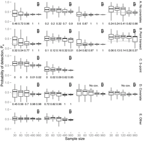
Fig. 3summarizes the estimates ofPaobtained if the candidate model set contains only mixture models (including 1-point mixtures); the numbers below each boxplot are the proportion of times the model selected by AIC was the model which generated the data.S1 Figshows the dis-tribution of estimates when only K+A models are used, giving a baseline to compare the mix-ture model results against (S2 Fig). Results using the recommended modelling strategy of both mixture and K+A models is shown inS2 Fig, and the number of times each model is chosen using the combined modelling strategy is shown inS3 Fig.

For Group A, the mixture approach produced unbiased results for scenarios A1 and A3 at all but the lowest sample size; even for then= 30 scenarios the bias was small, despite the cor-rect 2-point mixture model being selected only 46–60% of the time (Fig. 3—the half normal model was selected the remainder of the time). The K+A approach also performed well (S1 Fig). Unsurprisingly, therefore, the combined approach performed well (S2 Fig); what was a lit-tle surprising was that the correct model was only selected 60–76% of the time at the highest sample sizes for scenario A1, with the hazard-rate K+A model selected the remainder (S3 Fig). Scenarios A2 and A4 showed positive bias at smaller sample sizes under the mixture approach; bias reduced substantially by 480 observations, where a large proportion of the selected models were 2-point mixtures. Unlike scenarios A1 and A3, the detection functions in scenarios A2 and A4 were evidently not well approximated by a half-normal, and hence at lower sample sizes where the two point mixture tended not to be selected, the results were biased. The K+A approach did not fare well with these scenarios, showing strong positive bias even at the largest sample sizes. In combination, the mixture models were chosen over K+A models at larger sam-ple sizes, and so the combined modelling approach produced much better results than K +A alone.

As expected, results were worse for the point transect scenarios of Group B. Estimates from the mixture approach were biased at low sample sizes for B1, when the two-point model was rarely selected, but were unbiased given 120 observations and greater. Estimates for B3 were unbiased. For B2 and B4, results were positively biased at small sample sizes, just as with A2 and A4, but unlike the line transect scenarios the bias did not disappear even at the largest sam-ple size. This is unsurprising given the very small number of detections coming from the less detectable mixture component (seeFig. 2—the marginal pdf is almost identical to that of the easier to detect mixture component). Bias was generally worse with the K+A approach (S1 Fig), and the combined approach (S2 Fig) produced marginally better results than K+A alone; for scenarios B1 and B3 the combined results were much better than K+A alone.

preferred by AIC. In both cases, the K+A results were worse (S1 Fig), although they were not far from unbiased for C2. In the combined results, the mixture models were chosen most 52–68%) of the time for model C1, while for C2 the mixture models were chosen less often (15–60% of the time); despite this, the results were just as good as those using mixtures alone (S2 Fig).

We first address the results of the Group D simulations when covariates were available for inclusion in candidate models. Results for D1 were positively biased at lower sample sizes, but Fig 3. Simulation results: boxplots of the estimated average detection probabilities,Pa, for the best mixture model (by AIC score).Layout is as in Fig. 2. Grey lines indicate the true value of the average detection probability. Numbers underneath each boxplot give the proportion of AIC best models that were of the same form as the model that the data was simulated from (e.g., Scenario D1 the proportion of AIC best models that were 2-point mixtures that included the covariate in the model).

less so as the sample size increased, and almost unbiased by 120 observations, where the correct model was selected most of the time (Fig. 3). Results for D2 were close to unbiased at all sample sizes. Estimates from the K+A models were positively biased at almost all sample sizes for D1, and almost unbiased for D2 (S1 Fig).

When covariate information is not available for fitting the model, the mixture model detec-tion funcdetec-tions still performed well, showing that when covariates are not available mixture components can compensate, though not through using additional components (seeS3 Fig, 3-point mixtures are never AIC-best models). For the K+A models without covariates, perfor-mance was also similar to that from the covariate models, indicating that the flexibility provid-ed by the series adjustment can compensate for lack of covariate information in that

framework. However, results were still slightly biased even at large sample sizes (S1 Fig). As might be expected, bias was less when both approaches were combined (S2 Fig).

The Group E results were encouraging. Although the mixture formulation was biased even at large sample sizes, the bias was always small (Fig. 3), and generally no worse than that under the K+A formulation, which also showed a small bias (S1 Fig). We had anticipated good per-formance of the mixture models for scenario E1, since the detection function shape is not far from half-normal; however it was not obvious that performance would be good for E2, where the marginal shape cannot be approximated well by a mixture of half-normal functions. The combined strategy was no worse than either formulation alone in terms of bias.

Case studies results

British Columbia marine mammals. Results are summarised inTable 1and detection

functions for the AIC-best models are shown inFig. 4. In each case mixture models were two component models. For harbour seal, the mixture model had a lower AIC than for the K+A model reported in Williams and Thomas [20]. The mixture model^Pais approximately 20%

lower, implying that the previous estimate ofN^may have been an underestimate (asPa de-creases, 1/Paincreases in the Horvitz-Thompson estimator giving a larger estimate of abun-dance). For harbour porpoise, the mixture model AIC is almost 1.5 points higher than the K+A model, which was a hazard-rate with no adjustments. Hence, the model likelihoods are very similar, but the penalty due to the 2-point mixture having an additional parameter prevents it from being selected. The^Pafrom the two models are very close. Lastly, for humpback whales, the mixture model AIC is almost 3 points higher than the K+A model—however, one advan-tage of the mixture model is that the fitted function is monotone (Fig. 4) while the K+A func-tion is not (Fig. 1). Again, the estimatedP^as are very similar.

Long-finned pilot whales. A mixture model detection function was fitted with each

covar-iate, as well as a model with no covariates. The best model by AIC score (Table 1) was a 2-point mixture with Beaufort sea state included as a continuous covariate.Fig. 5shows the average de-tection function (in the sense that a dede-tection function was evaluated over the range (0,w) for each covariate combination and was then averaged point-wise) and the marginal detection function with the quartiles of Beaufort sea state. None of the non-monotonic behaviour seen in

Fig. 1can occur when a mixture is used.

Wood ants. All combinations of main effects were fitted (Table 1), and the best model by AIC was a 2-point mixture with nest size and habitat as covariates (S4 Fig). This model had an AIC that was considerably (6 points) lower than the AIC-best K+A model, a hazard-rate with the same covariates.^Pais about 10% lower when estimated using the mixture model.

Amakihi. The AIC-best mixture model was a two point mixture with observer and

covariates performed better than mixtures in AIC terms, although by less than 1 AIC point. The difference in^Pabetween these two models is about 15%. It is encouraging that there is such a small difference in AIC, and that covariate mixture models were selected over mixture models without covariates, despite the large number of parameters that such models entail.

Discussion

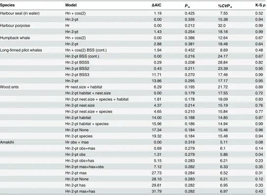
We have investigated and demonstrated the utility of detection functions constructed from mixtures of half-normal functions in both line and point transect distance sampling. We also Table 1. Comparison of case study analysis results.

Species Model _ΔAIC _P^_{a %CVP}^_a K-S_p

Harbour seal (in water) Hn + cos(2) 1.19 0.425 7.55 0.52

Hn 2-pt 0.00 0.335 15.38 0.94

Harbour porpoise Hr 0.00 0.212 32.0 0.99

Hn 2-pt 1.43 0.254 18.18 0.99

Humpback whale Hn + cos(2) 0.00 0.386 12.64 0.67

Hn 2-pt 2.88 0.381 18.48 0.64

Long-finned pilot whales Hn + cos(2) BSS (cont.) 1.94 0.452 8.69 0.48

Hn 2-pt BSS (cont.) 0.00 0.216 24.17 0.67

Hn 2-pt BSS5 0.29 0.208 28.84 0.82

Hn 2-pt BSS2 0.43 0.211 23.39 0.95

Hn 2-pt BSS3 11.71 0.270 17.46 0.99

Hn 2-pt 13.86 0.295 17.17 0.95

Wood ants Hr nest.size + habitat 6.29 0.195 21.72 0.89

Hn 2-pt habitat + nest.size 0.00 0.179 17.55 0.72

Hn 2-pt nest.size + species + habitat 1.81 0.178 18.09 0.83

Hn 2-pt nest.size 4.37 0.214 15.19 0.76

Hn 2-pt nest.size + species 4.65 0.210 15.84 0.77

Hn 2-pt habitat 14.00 0.188 14.85 0.97

Hn 2-pt habitat + species 15.96 0.186 14.94 0.99

Hn 2-pt None 17.34 0.184 15.46 0.96

Hn 2-pt species 19.32 0.184 15.48 0.94

Amakihi Hr obs + mas 0.00 0.319 5.11 0.08

Hn 2-pt obs+mas 0.69 0.279 6.1 0.14

Hn 2-pt obs 1.31 0.279 5.86 0.04

Hn 2-pt obs+has 5.15 0.283 6.21 0.23

Hn 2-pt mas+has+obs 7.12 0.282 6.33 0.35

Hn 2-pt mas 27.73 0.284 6.52 0.31

Hn 2-pt None 28.10 0.283 6.21 0.12

Hn 2-pt has 29.81 0.282 6.95 0.33

Hn 2-pt mas+has 31.79 0.282 6.97 0.43

Comparison of results from Williams and Thomas [20], Pike et al. [10], Borkin et al. [21] and Marques et al. [17] with results fromfitting mixture model detection functions. Table columns give case study species, modelfitted (In the table“(cont.)”denotes that the covariate was included in the model as continuous, otherwise covariates entered the model as factors; BBSn indicates Beaufort sea state withnfactors); cos(x) indicates a Cosine adjustment of orderx), difference in AIC from AIC-best model (denotes withΔAIC = 0), average detectability, percentage coefficient of variation in average detectability andp-value from a Kolmogorov-Smirnov goodness-of-fit test. In each case thefirst line for each data set is the model from the original article and the subsequent models are inΔAIC order. Mixture model components were selected by AIC (ΔAIC from best model is listed).

show that covariates can be readily included in such models. Further, these mixture detection functions can be simply“dropped into”other extensions of conventional distance sampling such as: methods for dealing with incomplete detection at zero distance [22,23] (for these models, there is an additional mark-recapture component to the likelihood, where mixture models could also be used, as in [11–14]), spatial models for distance sampling data [24,25] or models for surveys where distances were measured with error [26]. Though we were necessarily Fig 4. Plots of the mixture model detection functions fit to the British Columbia marine mammal data.In each case the best mixture model by AIC was a 2-point mixture. Dashed lines show the mixture components.

doi:10.1371/journal.pone.0118726.g004

limited to only a few example data sets on specific taxa, we note that there is no limitation to the species or survey setup that mixture model detection functions can be used with.

We have shown that the mixture models perform well on both simulated and survey data where traditional methods produce suboptimal results. In many cases the proposed model out-performed K+A models in AIC terms, which is surprising given that the mixture models in question often had more parameters. In particular mixture model detection functions appear useful when dealing with line transect data that has a spike in detection probability at small dis-tances, though we note that it is better to avoid collecting such data in the first place, where possible ([1], p. 42) (spikes are commonly caused by observers spending too much effort near the trackline/point and not looking further afield). Also, other non-detection-related factors can cause a spike, such as rounding of measurements or responsive animal movement, and if present in the data these should be dealt with using other analysis strategies or field methods [1]. For line transect surveys, unbiased estimation ofPawas possible even for very spiked detec-tion funcdetec-tions, so long as the sample size of observadetec-tions was large (Scenarios A2 and A4). By contrast, estimates remained badly biased at all sample sizes for the equivalent point transect scenarios (B2 and B4). For such surveys, where such a small proportion of the data comes from the closer distances, then perhaps the only effective solution is to constrain the fit, for example using a Bayesian approach with strong priors on the detection function parameters.

We note that in our case studies, a larger coefficient of variation in the average detectability was reported with mixtures than with half-normal K+A models but mixtures seemed to have lower CVs (again, of^Pa) than hazard-rate K+A models (in the line transect case, ignoring

non-monotonic K+A models; seeTable 1). This can be explained by considering the flexibility of the detection function. A half-normal detection function is relatively inflexible so uncertainty is low (since there is only one parameter and it only affects the scale of the function). However, for a hazard-rate model the shoulder can vary from very small (spiked) to very large (depend-ing on the shape parameter), so the uncertainty in this more flexible model is larger. Mixtures of half-normals lie somewhere in between these two options (only the scales change which are weighted, we are then summing smaller variances).

Simulations show that small sample sizes do not support the use of mixture models with a high number of components, even when the data were generated from such a model. We avoid poorly fitting models of this sort by using both K+A and mixture detection functions and se-lecting the best between them (comparingFig. 3withS1 Fig). This integrated approach is builds upon current model selection procedures for a detection function analysis—currently se-lection is made between different K+A formulations and number of adjustment terms using AIC; mixture models simply add another alternative detection function where rather than ad-justment terms, mixture components are selected. So existing key-only models are special cases of the mixture detection functions.

In simulation we observed that 3-point mixture did not act as good surrogates for missing covariate information; 2-point mixtures were generally chosen by AIC (though these 2-point models performed well at higher sample sizes). In our case studies, 2-point mixtures consis-tently provided the best fit. Only examination of further data will show whether 3-point and higher mixtures can be supported, however we note that when the K+A series formulation is used, detection functions with 5 or more parameters are rarely selected by AIC (a 3-point mix-ture with no covariates requires 5 parameters). These results echo those in capmix-ture-recapmix-ture literature [11], where often only 2 component mixtures were selected.

are aware, all current alternatives fail some of the criteria given in the introduction—for exam-ple, the kernel functions can be non-monotonic. Giammarino & Quatto [28] have proposed a

“mixture model”detection function—their model takes a rather different form to the mixtures we describe here (simply exp(−x2/(2σ2))−x/τ)), though their results indicate there is little dif-ference between their model and K+A approaches.

The mixture component used here was a half-normal, but other component functions may prove useful. In particular, a mixture of hazard-rate functions with different shape and/or scale parameters for each component may be better at fitting detection functions with a wide shoul-der, a steep drop-off and then a second plateau in detectability (see E2 inFig. 2, which was gen-erated from a mixture of two hazard-rate functions). Further, a mixture of a half-normal (or hazard-rate) and a uniform kernel may prove useful—this would have only two (or three) pa-rameters, and hence may be more competitive (in AIC terms) with K+A models.

Another potentially useful extension is continuous mixtures of the form

gðxÞ ¼

Z

Rφ

ðkÞg_kðx;Z;θ;kÞdk

whereφ(κ) is a weighting function that controls the mixing ofgκ. Provided that an appropriate

function can be chosen forφ, moreflexible models could be used whilst keeping the number of parameters low. In addition, a combination of bothfinite and continuous mixtures could be used, echoing the work in capture-recapture [14]. Such models require more complex optimi-sation procedures in order to estimate their parameters in a maximum likelihood context, though are well suited to a Bayesian setting.

Mixture model detection functions based on half-normal components are available as an R package, mmds, which is available on CRAN. These models will be added to the next version of the Distance for Windows software and the R package Distance.

Supporting Information

S1 Appendix. Optimization details.

(PDF)

S2 Appendix. Simulation parameters.

(PDF)

S1 Text. Derivatives of the likelihood.

(PDF)

S2 Text. Variance estimation for mixture model detection functions.

(PDF)

S1 Fig. Simulation results: boxplots of the estimated average detection probabilities,Pa, for the best K+A model (by AIC score).Grey lines indicate the true value of the average

detection probability. (EPS)

S2 Fig. Simulation results: boxplots of the estimated average detection probabilities,P_a, for

the best model (by AIC score) for both mixture and K+A models.In each case the best

proportion of times that the AIC best model was a 2- or 3-point mixture model. (EPS)

S3 Fig. Simulation results: stacked bar charts showing the number of models selected by AIC that fall into the given model classes.Layout is as inS2 Fig.“hn”is a half-normal detec-tion funcdetec-tion (i.e. 1-point mixture) and“hr”is a hazard-rate detection function (no adjust-ments). K+A indicates a key function plus adjustment term model where“cos”is cosine and

“poly”are simple polynomial adjustments. MMDS is a mixture model with 2 or 3 components (“2-pt”or“3-pt”, respectively).“(cov)”indicates that covariates were included in the model. (EPS)

S4 Fig. Plot of the detection functions for the AIC best model for the ants data set (2-point mixture with nest size and habitat as covariates).The first panel shows the average detection function (dashed lines are the two mixture components of the detection function, averaged over covariate values). The second and third panels show the quartiles of nest size and the lev-els of habitat type respectively.

(EPS)

S5 Fig. Plots of the (AIC) best mixture model for the Amakihi data: a 2-point mixture with observer and minutes after sunrise as covariates.Top row: detection function averaged over covariates (dashed lines are each mixture component averaged over covariates), marginal de-tection function showing the levels of observer (averaged over the values of minutes after sun-rise) and marginal detection function for minutes after sunrise ranging between 0 and 300 minutes (averaged over the levels of observer), as in Marques et al (2007) [17]. Bottom row: pdf of distances averaged over the covariate values.

(EPS)

Acknowledgments

DLM acknowledges the UK Engineering and Physical Sciences Research Council for financial support during his PhD, and Simon Wood for useful discussions. Both authors thank David Borchers, who suggested the parametrisation for the mixture proportions (S1 Appendix) and Tiago Marques for helpful comments on an earlier draft. The authors also wish to thank Rain-coast Conservation Foundation and Rob Williams for allowing the use of perpendicular sight-ings distance data previously reported in [20]; Daniel Pike, Gísli Vikingsson and Bjarni Mikkelsen at the Marine Research Institute, Iceland for the long-finned pilot whales data; Kerry Borkin for the wood ant data and Steven Fancy for the use of the Amakihi data.

Author Contributions

Conceived and designed the experiments: DLM LT. Performed the experiments: DLM. Ana-lyzed the data: DLM. Contributed reagents/materials/analysis tools: DLM. Wrote the paper: DLM LT. Designed the software used in analysis: DLM LT.

References

1. Buckland ST, Anderson DR, Burnham KP, Laake JL, Borchers DL, et al. (2001) Introduction to Distance Sampling. Oxford University Press.

2. Buckland ST, Anderson DR, Burnham KP, Laake JL, Borchers DL, et al. (2004) Advanced Distance Sampling. Oxford University Press.

4. Thomas L, Buckland ST, Rexstad EA, Laake JL, Strindberg S, et al. (2010) Distance software: design and analysis of distance sampling surveys for estimating population size. Journal of Applied Ecology 47: 5–14. doi:10.1111/j.1365-2664.2009.01737.xPMID:20383262

5. R Core Team (2013) R: A Language and Environment for Statistical Computing. Vienna, Austria. URL http://www.R-project.org/.

6. Laake JL, Borchers DL, Thomas L, Miller DL, Bishop JR (2014) mrds: Mark-Recapture Distance Sam-pling (mrds). URLhttp://CRAN.R-project.org/package = mrds. R package version 2.1.6.

7. Marques F, Buckland ST (2003) Incorporating covariates into standard line transect analyses. Bio-metrics 59: 924–935. doi:10.1111/j.0006-341X.2003.00107.xPMID:14969471

8. Schittkowski K (1986) NLPQL: A Fortran subroutine for solving constrained nonlinear programming problems. Annals of Operations Research 5: 485–500. doi:10.1007/BF02022087

9. Ye Y (1987) Interior Algorithms for Linear, Quadratic, and Linearly Constrained Convex Programming. Ph.D. thesis, Stanford University.

10. Pike DG, Gunnlaugsson T, Vikingsson AG, Desportes G, Mikkelson B (2003) An estimate of the abun-dance of long-finned pilot whales globicephala melas from the NASS-2001 shipboard survey. Technical Report SC/11/AE/10.

11. Pledger S (2000) Unified maximum likelihood estimates for closed capture-recapture models using mix-tures. Biometrics 56: 434_–442. doi:10.1111/j.0006-341X.2000.00434.xPMID:10877301

12. Dorazio RM, Royle JA (2003) Mixture models for estimating the size of a closed population when cap-ture rates vary among individuals. Biometrics 59: 351–364. doi:10.1111/1541-0420.00042PMID: 12926720

13. Pledger S (2005) The performance of mixture models in heterogeneous closed population capture-re-capture. Biometrics 61: 868–873. doi:10.1111/j.1541-020X.2005.00411_1.xPMID:16135042 14. Morgan BJT, Ridout MS (2008) A new mixture model for capture heterogeneity. Journal of the Royal

Statistical Society Series C: Applied Statistics 57: 433–446. doi:10.1111/j.1467-9876.2008.00620.x 15. Link W (2003) Nonidentifiability of population size from capture-recapture data with heterogeneous

de-tection probabilities. Biometrics 59: 1123–1130. doi:10.1111/j.0006-341X.2003.00129.xPMID: 14969493

16. Miller DL (2011) mmds: Mixture Model Distance Sampling (mmds). URLhttp://CRAN.R-project.org/ package = mmds. R package version 1.1.

17. Marques TA, Thomas L, Fancy S, Buckland ST (2007) Improving estimates of bird density using multi-ple-covariate distance sampling. The Auk 124: 1229_–1243. doi:10.1642/0004-8038(2007)124% 5B1229:IEOBDU%5D2.0.CO;2

18. Otto MC, Pollock KH (1990) Size Bias in Line Transect Sampling: A Field Test. Biometrics 46: 239– 245. doi:10.2307/2531648

19. Miller DL (2014) Distance: A simple way to fit detection functions to distance sampling data and calcu-late abundance/density for biological populations. URLhttp://CRAN.R-project.org/package = Distance. R package version 0.6.1.

20. Williams R, Thomas L (2007) Distribution and abundance of marine mammals in the coastal waters of British Columbia, Canada. Journal of Cetacean Research and Management 9: 15.

21. Borkin KM, Summers RW, Thomas L (2012) Surveying abundance and stand type associations of For-mica aquiloniaandF. lugubris(Hymenoptera: Formicidae) nest mounds over an extensive area: Trial-ing a novel method. European Journal of Entomology 109: 47–53. doi:10.14411/eje.2012.007 22. Laake JL, Borchers DL (2004) Methods for incomplete detection at zero distance. In: Buckland ST,

an-derson DR, Burnham KP, Laake JL, Borchers DL, et al., editors, Advanced Distance Sampling, Oxford University Press. pp. 48–70.

23. Laake JL, Collier BA, Morrison ML, Wilkins RN (2011) Point-based mark-recapture distance sampling. Journal of Agricultural, Biological, and Environmental Statistics 16: 389–408. doi: 10.1007/s13253-011-0059-5

24. Hedley SL, Buckland ST (2004) Spatial models for line transect sampling. Journal of Agricultural, Bio-logical, and Environmental Statistics 9: 181–199. doi:10.1198/1085711043578

25. Miller DL, Burt ML, Rexstad EA, Thomas L (2013) Spatial models for distance sampling data: recent de-velopments and future directions. Methods in Ecology and Evolution 4: 1001–1010. doi:10.1111/ 2041-210X.12105

27. Eidous O, Shakhatreh MK (2011) Asymptotic Unbiased Kernel Estimator for Line Transect Sampling. Communications in Statistics—Theory and Methods 40: 4353–4363. doi:10.1080/03610926.2010. 510253