regions. In order to investigate the line profiles from dynamical collapsing massive star-forming regions (MSFRs), we model the emission from hydrodynamic simulations of a collapsing cloud in the absence of outflows. By performing radiative transfer calculations, we compute the optically thick HCO+ and optically thin N2H+ line profiles from two collapsing regions at different epochs. Due to large-scale collapse, the MSFRs have large velocity gradients, reaching up to 20 km s−1pc−1across the central core. The optically thin lines typically contain multiple velocity components resulting from the superposition of numerous density peaks along the line of sight. The optically thick lines are only marginally shifted to the blue side of the optically thin line profiles, and frequently do not have a central depression in their profiles due to self-absorption. As the regions evolve, the lines become brighter and the optically thick lines become broader. The lower-order HCO+(1–0) transitions are better indicators of collapse than the higher-order (4–3) transitions. We also investigate how the beam sizes affect profile shapes. Smaller beams lead to brighter and narrower lines that are more skewed to the blue in HCO+relative to the true core velocity, but show multiple components in N2H+. High-resolution observations (e.g., with Atacama Large Millimeter Array) can test these predictions and provide insights into the nature of MSFRs.
Key words: line: profiles – stars: formation – stars: massive
Online-only material:color figures
1. INTRODUCTION
The birth of massive stars is inextricably linked to that of cluster formation, as most massive stars form at the center of dense molecular clouds. The structure of such regions is dense and filamentary, far removed from simple spherical models. In Smith et al. (2012), hereafter Paper I, we investigated the line profiles that would be observed from collapsing cores embedded within filaments from simulations of clustered star formation. We found that the dense filaments frequently obscured the collapsing core and a blue asymmetric collapse profile (Zhou 1992; Walker et al.1994; Myers et al.1996) was observed in less than 50% of sightlines. In the current paper, we extend this analysis to study the line profiles produced during the initial collapse of massive star-forming regions (MSFRs).
There have been numerous observational studies of line profiles from MSFRs (e.g., Wu & Evans2003; Fuller et al.2005; Wu et al.2007; Sun & Gao2009; Chen et al.2010; Csengeri et al. 2011a). Generally such studies have focused on finding infall candidates by identifying blue asymmetries in their optically thick lines (seePaper Ior the review by Evans1999.) A common way of classifying such surveys is using the blue excess seen across the survey, i.e., the number of blue biased profiles minus the number of red biased profiles divided by the total number of observations (Mardones et al.1997). Typical values for such surveys are around 10%–30%. This finding could be interpreted in several ways. First, the majority of MSFRs could be quasi-equilibrium objects containing static massive pre-stellar cores that have not yet collapsed (Tan et al. 2006). Alternatively, most MSFRs could be collapsing according to their dynamical timescale (Elmegreen2000; V´azquez-Semadeni et al.2005) but
the observational signature produced differs from that predicted by simple spherical models. There are alternative models of massive star formation in which massive stars are formed from well defined massive pre-stellar cores supported by super-sonic turbulence (McKee & Tan 2003), however predictions of the observed line profiles resulting from such theories have not yet been calculated.
In this paper, we use the simulations presented in Smith et al. (2009), hereafter S09, in which a cluster of low-mass stars are formed around massive ones to investigate the observational signatures of a collapsing MSFR. We consider the case where the MSFR has already formed a protostar at its center which is growing rapidly in mass through accretion. This simulation follows the competitive accretion formalism (Bonnell et al. 2003,2004; Bonnell & Bate2006) in which massive stars are formed at the center of a collapsing cluster where the cluster potential funnels gas toward the massive protostar (see also Klessen & Burkert2000; Girichidis et al.2011).
These simulations lack outflows, which are known to affect HCO+line profiles (Rawlings et al.2004). To this end we will focus our modeling on the earliest stages of the collapse before outflows become significant. Without first considering the sim-ple dynamical case without inflows, it would be impossible to disentangle the two effects. Despite this, we will compare our results to observational studies, that may have outflows present, in order to understand to what extent the dynamics of a com-plex clustered star formation region can explain observed line profiles.
Table 1
The Mass Contained within Each Region When the Central Sink Mass is of Order 0.5Mand 5.0M
Region Central Sink Gas Mass Total number Final Sink
Mass (M) (M) of Sinks Mass (M)
A 0.5 370 36 29.2
B 0.7 257 11 10.7
A 5.4 354 73 29.2
B 5.0 260 18 10.7
Notes.The gas mass excludes the mass in sinks. The final sink mass corresponds to the mass of the central sink when the simulation is terminated.
of the simulated observations and then directly compares the profiles to observations. We discuss some qualifications and compare to low-mass star formation in Sections 4.1 and 5. Section6provides a summary.
2. METHOD
As inPaper I, we use the radiative transfer code RADMC-3D (Dullemond 2012) to calculate the line profiles from star-forming regions extracted from the simulations ofS09. These simulations followed the evolution of a 104M
cylindrical
giant molecular cloud as it undergoes star formation using the smoothed particle hydrodynamic method (Monaghan 1992). Several massive stars were formed at the center of clusters. Our line transfer utilizes the large velocity gradient proposed by Sobolev (1957), with the inclusion of “Doppler catching” to interpolate under-resolved velocities as implemented in RADMC-3D by Shetty et al. (2011a,2011b). In this section we highlight only the differences in our method from the previous paper, and for a full description of our methods we refer to Paper I.
The modeled regions are chosen from Smith et al. (2009) by finding the most massive sink particles and then selecting a 0.4 pc radius region around them. Sink particles represent sites of star formation and are formed from high-density gravitationally bound gas in the simulation (Bate et al.1995). The sink particles have a radius of 20 AU and it is possible that within this a multiple system is formed, however we shall use the term sink and protostar synonymously in what follows. We identify two independent regions, one of which forms a very massive sink particle (∼30M) and the other a less massive sink (∼10M).
One of our chosen species, HCO+, has been shown to be present in outflows (Rawlings et al.2004; Paron et al.2012). As we lack this physics in our simulation we concentrate on the early evolution of the MSFRs before outflows become dominant. We discuss potential implications of outflows in Section4.2.
The regions are considered at two epochs during their evolution, when the central sources are around 0.5M and 5.0M, corresponding to early and more evolved phases. The most massive sink reaches a final mass of around 30Mwhen the simulation is terminated. Table1outlines the properties of the two star-forming regions. In addition to the central massive protostar, multiple additional sites of star formation are also contained within the regions.
[image:2.612.43.295.85.163.2]In contrast to Paper I where we considered HCN as the optically thick tracer, for the MSFRs we use HCO+ due to the greater prevalence of observational studies of massive star formation using this species (e.g. Fuller et al. 2005; Csengeri et al. 2011a). We adopt a constant abundance of
Figure 1.Gas temperature along a line of sight directly through the central source when it has a mass of 5.0Mintegrated over a 0.06 pc FWHM beam. The temperature rises at the center due to heating from the sink particle representing the massive protostar.
AHCO+ =5.0×10⁻⁹relative to the H2number density (Aikawa
et al. 2005). For the optically thin tracer we adopt an N2H+ abundanceAN2H+ =10−10relative to H2(Aikawa et al.2005),
as inPaper I. We focus our analysis on the isolated hyperfine component (F101-012) at 93176.2527 MHz, which is displaced by 2.297 MHz from the neighboring hyperfine lines (Keto & Rybicki2010). Initially, we consider only the (1–0) transitions but later in the paper we shall compare to higher-order optically thick lines that trace higher densities due to their larger critical density. These two species are easily observable with the Atacama Large Millimeter Array (ALMA).
There is some suggestion that in real molecular clouds HCO+ and N2H+ abundances may be anti-correlated as HCO+ is depleted onto dust grains at low temperatures (e.g., Jørgensen et al. 2004). However, in massive star formation regions the temperatures around the central protostar are of order 20 K or higher, so freeze out should not be a major factor. In the simulated cloud, gas temperatures are calculated using a barytropic equation of state with an additional heating term from sinks based on the young stellar object models of Robitaille et al. (2006). The method is described in full in Smith et al. (2009). Figure1illustrates the effect of this heating along the simulated beam in the extreme case when the central sink in Region A has a mass of 5.0M. Along the line of sight the temperature is highest at the peak density where the sink particle heats the gas, but also increases toward the outside of the region where the gas is diffuse and would be heated by external radiation. As emission is dependent on both density and temperature, the line profiles are dominated by emission from the central source.
Figure 2.Density (grayscale) and velocity field (vectors) of two slices through the central source in Regions A and B. In Region A, there is a large-scale velocity gradient toward the central massive star. In Region B, this is also true of the majority of the dense gas but there are also indications of the background velocity flows that formed the dense filaments in which the massive star is embedded.
3. RESULTS
3.1. Velocity Fields
3.1.1. Simulation
For a full analysis of the dynamics of the MSFRs, seeS09. Here, we provide an overview of the underlying velocity fields in the simulated MSFRs.
Figure2shows the density and velocity in two slices through Regions A and B. The fields are normalized so that the most massive protostar has a position and velocity of zero. The main feature of the velocity fields is a large-scale infall motion toward the central object. As discussed in S09 it is this large-scale collapse of gas toward the central object that allows a massive star to form. However, there are a few additional features to note. In Region A, the massive star forms at the center of a
network of converging filaments, as predicted by Myers (2011), and the velocity vectors follow the contours of the filament toward the center. In Region B, there is evidence of the original velocity field of converging flows which formed the filaments in which the MSFR is embedded. The velocity field in the MSFR is therefore a combination of large-scale turbulent motions and gravitational collapse. This leads to a coherent velocity field over the box, which is in strong contrast to the lower-mass star formation studied in Paper I where the velocity field is extremely inhomogeneous. Additionally, it should be noted that unlike conventional models of spherically collapsing cores there is no envelope of static gas that surrounds the region.
associated with gas over-density. Figure 3 shows the density and velocity field along the x-axis of Region A. There are multiple peaks in the density field each of which contributes to the overall emission separately. Local maxima in the velocity field are associated with sites of small-scale collapse, however these are superimposed on top of a larger supersonic flow of a few km s−1 toward the core center from each direction. This velocity flow abruptly changes from positive to negative over the center of the region, where the massive star forms, with a gradient of more than 2 km s−1occurring in less than 0.1 pc.
3.1.2. Observations
Evidence for large-scale infall in massive star formation has been presented by a number of authors. In particular, Motte et al. (2007) carried out a survey of Cygnus X searching for massive pre-stellar cores. The authors did not find any truly pre-stellar cores but instead observed large-scale supersonic flows directed toward the centers of suspected young MSFRs. Further, Peretto et al. (2006,2007) found that the massive cluster-forming clump NGC 264-C was collapsing along its axis in accordance with its dynamical timescale, and therefore channeling mass toward the Class 0 object at its center. The violent collapse of gas to form high-mass protostellar objects was also proposed by Beuther et al. (2002) to explain their observed line widths and multiple velocity components.
Another similarity between these simulations and observa-tions is the prevalence of filamentary structure. A recent study by Peretto et al. (2012) of the Pipe nebula found the only indica-tion of star cluster formaindica-tion occurred at a point of convergence of multiple filaments. Similarly, Schneider et al. (2012) found cluster formation at the junction of filaments in the Rosette molecular cloud.
3.2. Optically Thin Profiles
3.2.1. Simulation
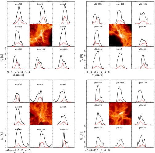
Figure 4 shows the modeled line profiles along various viewing angles through the central source in Regions A and B when the sink has a mass of ∼0.5M. In the left panels of the figures, the model is fixed atφ =0◦, and we view the model at 45◦ intervals in inclination. In the right panels, the inclination is fixed at inc=90◦, and we view the model at 45◦ intervals in rotation. We sample a total of 14 unique lines of sight through each core center. The red line shows the isolated N2H+1–0 hyperfine line multiplied by a factor of four so that it is visible alongside the HCO+(1–0) line (black). The most striking feature of the optically thin lines is that all the line profiles exhibit non-Gaussian features.
[image:4.612.320.568.52.295.2]In Section3.1, we demonstrated that the velocity field of the region is dominated by large-scale infall motions but the density field contains multiple peaks. Figure 5 shows the N2H+ line profile resulting from integrating the emission along the line of sight shown in Figure3, with a two component Gaussian fit shown in red. There are major components at velocities +1.5 km s−1and 0 km s−1, with the latter containing additional substructure. An examination of Figure3shows that most of the material on one side of the central protostar is collapsing toward the center at a roughly constant velocity +1.5 km s−1 and that the gas traveling at this velocity contains a number of dense cores. The aggregate emission from these cores produces the line peak at this velocity. The velocity field of the region is normalized such that the central protostar has a velocity of zero, resulting in the second Gaussian component peaking at
Figure 3.Gas density and velocity along a line of sight directly along thex-axis of Region A. The quantities are averaged over a Gaussian beam of 0.06 pc FWHM. There is a large velocity gradient over the point where the massive star forms, and the density field shows considerable substructure.
this velocity. Figure 3shows that the density field around the core is not smooth as there are dense knots of gas at either side of the core, each with a slightly different velocity. This results in the two maxima in the velocity profile in this component.
Further examination of the components of the N2H+ lines in Figure4indicates that each peak in the optically thin lines comes from a knot of dense gas in the MSFR. In our simulations, MSFRs are also cluster-forming regions (Bonnell et al. 2004; Bonnell & Bate2006; Smith et al.2009). Such regions contain many cores of dense gas, all of which emit strongly in N2H+ (1–0) at a velocity determined by the local speed at which gas is collapsing toward the center. This is not true just of the simulations used here; Krumholz & Tan (2007), Krumholz et al. (2009), and Girichidis et al. (2012) also find multiple cores of dense gas in MSFRs.
We note that multiple components in a line profile can also be attributed to optical depth effects, and while N2H+ is generally optically thin, it may become optically thick in the densest regions of the core. In Figure 4, it is immediately apparent that optical depth effects are not causing the multiple components in the lines as the N2H+ profiles are symmetric through 180◦, an impossible outcome if the lines were optically thick. Observationally, either an estimation of the optical depth or complementary observations of another optically thin species would be required to confirm that multiple components in a line profile arise from substructure.
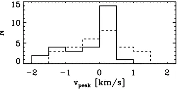
Another interesting feature of the optically thin emission from our MSFRs is that the line peak does not always correspond to the velocity of the massive protostar. Figure6shows a histogram corresponding to the N2H+line peak for all the viewing angles in Figure 4. The peak is frequently displaced by more than 0.5 km s−1from the velocity of the massive protostar.
Figure 4.HCO+(1–0) black and N2H+(1–0) red line profiles from Regions A (top) and B (bottom). The N2H+(1–0) is multiplied by a factor of 4 in order to be visible. The central color image shows the column density in the plane in which the sight-lines pass through the core, and the position at which the outer panels touch the central image indicates the orientation of the sightline. The line profiles are calculated for a 0.06 pc beam centered directly on the embedded core. The central box has a physical size of 0.8 pc. In the left panels the declination angle has a constant value ofφ=0◦, and in the right panels the inclination has a constant value of inc=90◦. Note that the N2H+lines are symmetric through 180◦as they are optically thin.
(A color version of this figure is available in the online journal.)
3.2.2. Observations
While such non-Gaussianity is not observed in low-mass star formation, recent studies of high-mass star formation have de-tected multiple components from high-resolution interferometer observations of cloud centers. For example, Beuther et al. (2013) present an analysis of the starless prospective MSFR region IRDC18310-4 in which multiple components are clearly ob-served in N2H+(1–0) lines at the location of some of the 870μm peaks. Csengeri et al. (2011b) carried out a high-resolution dy-namical study of the massive clump DR21(OH) and found that
while single dish N2H+(1–0) observations reveal a single com-ponent, the line splits into multiple components when observed with an interferometer. This effect was particularly clear when observing the massive dense cores in the region. Multiple N2H+ (1–0) peaks can also be seen in some cases of Fuller et al. (2005) although in this case the regions are more poorly resolved com-pared to those studied here, an issue we will discuss in more detail later.
Figure 5.N2H+ (1–0) F(2–1) line profile from Region A when viewed at
i=90◦φ=90◦. The red line shows a simple two component Gaussian fit to the emission. The line has multiple velocity components due to a number of dense cores along the line of sight.
(A color version of this figure is available in the online journal.)
Figure 6.Velocity corresponding to the peak HCO+(1–0) (solid) and N2H+ (1–0) F(2–1) (dashed) emission from all simulated lines of sight. The distribution of optically thick line peaks has a blue excess relative to the optically thin peaks.
dense cores in MSFRs (Bontemps et al.2010; Longmore et al. 2011; Rod´on et al.2012), suggesting that non-Gaussian optically thin lines should be a feature of massive star formation.
3.3. Optically Thick Profiles
3.3.1. Simulation
Figure4shows the observed line profiles at various viewing angles through the central source in Regions A and B when it has a mass of around 0.5M. The optically thick HCO+(1–0) line is shown by the black line. The majority of the lines have a greater peak emission on their blue side than the red. As was shown by Zhou (1992) and Myers et al. (1996) a double peaked profile with an excess of emission on the blue side is an indication of collapse (seePaper Ifor a detailed discussion). The profiles presented here do not always show this classical two peaked signature, but there is usually brighter emission on the blue side. The optically thick line profiles characteristically resemble a saw tooth with a sharp rise in emission on the blue side followed by a more gradual drop off and in some cases a red shoulder.
[image:6.612.60.281.52.218.2] [image:6.612.317.571.87.133.2]This signature is qualitatively rather insensitive to viewing angle, although in quantitative terms there are noticeable vari-ations. In Region A, collapse occurs over a very wide volume and consequently there is a peak toward the blue side in most profiles. In Region B, which forms a less massive star, the infall profiles show a greater degree of variability reflecting the fact that the inward motions are less pronounced. Still the majority of lines show a blue excess.
Table 2
The Number of Cases Where the Offset in km s−1between the Optically Thick and Thin (1–0) Emission is of a Given Magnitude
Offset <−1.0 <−0.5 <0.0 >0.0 >0.5 >1.0
All 3 11 19 9 1 1
Single 1 6 15 3 1 1
Notes.We consider two samples. First, the full sample where all sightlines are included. In this case, the offset is between the location of the peak optically thick and thin emission. Second, we consider only those sightlines where the optically thin emission has no clear secondary component. In this case, the offset is between the location of the peak optically thick emission and the central velocity of a Gaussian fit to the optically thin emission. Our sample contains 28 lines in total.
A more quantitative estimate of the asymmetry of the line is usually given by the normalized velocity differenceδV between the optically thick and thin components (Mardones et al.1997). However, as discussed in Section 3.2since the optically thin lines cannot be consistently fit by one single component, this analysis is technically no longer valid. Nonetheless, a blue excess is seen in the optically thick lines. Figure6shows the histogram of the peak velocities in the HCO+(1–0) lines. They are clearly shifted to the blue side relative to the N2H+(1–0) peak velocities. In 19 out of 28 cases, the peak emission in HCO+(1–0) occurs toward the blueward side of the N
2H+(1–0) peak.
Table 2 summarizes the offsets in position between the optically thin and thick emission peaks. Table 2 utilizes two samples. First, the full sample used to produce Figure6, which includes cases where the N2H+ (1–0) emission had multiple components. Second, the subset of the sightlines that had only a single component in N2H+(1–0). In order to determine whether a sightline should be included we ignored small variations in the line profile that would be hidden by noise in a true observation, but excluded cases where there was clearly more than one major component. In this case, the rest velocity of the N2H+emission was determined by fitting a Gaussian to the profile. When compared to the typical widths of the line (several km s−1) the offsets are not very large. Mardones et al. (1997) required that the offset between the optically thick and thin emission be more than 0.25 times the line width of the optically thin component to certify a line as having a blue excess. Fuller et al. (2005) found N2H+line widths of order 2 km s−1in their sample meaning that we should require an offset of more than−0.5 km s−1to classify a core as having a blue excess. Only 11 out of 28 of the HCO+ (1–0) emission lines have an offset of more than−0.5 km s−1 indicating that more than half of our line profiles would not be considered infall candidates if these stricter criteria were adopted. When we exclude line profiles with multiple N2H+ components this falls to 6 out of 18 remaining profiles.
Our sample has a blue excess of onlyE=(NB−NR)/NT = (11–1)/28 =0.36NB andNR are the number of red and blue
profiles, andNTis the total number of profiles. The excess falls
to 0.18 if we require the N2H+ to have a single component. This small excess occurs despite the fact that both regions are collapsing so an excess of E = 1.0 would be expected when considering all viewing angles.
[image:6.612.80.260.285.376.2]Figure 7.Evolution of a line profile as the central object grows in mass in Region A. The left panel shows a central mass of 0.5Mand the right a central mass of 5.0M. The black line shows the HCO+(1–0) emission and the red line the N2H+(1–0) F(2–1) emission multiplied by a factor of four so that it is visible in the plot. Over time the line gets brighter and wider.
(A color version of this figure is available in the online journal.)
peaked line profile relies on a collapsing region having two points at a given velocity, one at the center of the core and the other at the outside. In Region A, the outer extents of the MSFR are flowing inward with supersonic velocities of±1.5 km s−1. Consequently, at velocities of ±1 km s−1 there is no self-absorption from gas in the outer regions and consequently all the emission from the center of the region where the massive star forms is visible. This probably also accounts for the modest displacement between the optically thick and thin peaks. When compared to monolithic collapse with a static envelope, infall signatures should be much more difficult to detect in a chaotic cluster formation scenario.
3.3.2. Observations
Detecting infall toward of MSFRs has been the focus of various observational studies (e.g., Wu & Evans2003; Sun & Gao2009; Chen et al.2010). We focus here on just two such studies: Fuller et al. (2005), which is a large-scale search for infall motions, and Csengeri et al. (2011a) which is amongst the most highly resolved observations to date.
Fuller et al. (2005) carried out a molecular line survey toward 77 candidate high-mass protostars and identified 21 infall candidates, showing blue asymmetry in their HCO+(1–0) lines, and 11 red profiles. The blue excess was calculated using the method of Mardones et al. (1997). The simulated observations presented here also have a large blue excess, but a greater fraction of the lines are blue and there are fewer red asymmetries. The latter is easily explained by the lack of outflows in our simulations, which could easily increase the number of red asymmetries. Another factor is that Fuller et al. (2005) used a larger beam than we consider in these simulations. We will show in Section3.6that this reduces the strength of the blue asymmetry. A third factor is that the blue asymmetry we observe is typically quite small in magnitude, this raises the possibility that some of the Fuller et al. (2005) cores with only a slight blue excess may also be collapsing.
[image:7.612.45.293.55.223.2]Csengeri et al. (2011a) carried out a survey of young dense cores in Cygnus X that showed the cores were dynamically evolving objects. The authors fit their observed line profiles to a model of a collapsing spherical core to estimate key properties.
Figure 8.As in Figure7but for Region B. The rise in N2H+emission at the right edges of the plots is the neighboring hyperfine line.
(A color version of this figure is available in the online journal.)
Table 3
Line Widths and Peak Line Intensities
Region Species 0.5M 5.0M
Ipeak(K) v95%(km s−1) Ipeak v95%
A N2H+ 0.57 3.31 0.36 4.19
B N2H+ 0.36 3.14 0.32 4.28
A HCO+ 6.27 3.95 8.60 5.05
B HCO+ 4.63 4.39 7.59 5.43
Notes.The peak line intensity, and line width within which 95% of the emission is contained for the simulated line profiles. This is calculated when the central source has a mass of 0.5Mand 5.0M, respectively.
This model predicts that each core should have a central absorption dip. However, the observed line profiles frequently did not show this feature, suggestive of large-scale infall without a static envelope, as found in our simulated models.
3.4. Time Evolution
3.4.1. Simulation
A further consideration is the evolution of such massive cores, as obviously not all regions will be observed when the central protostar has a mass of 0.5M as modeled above. Figures 7 and8show the evolution of the line profile observed ati =0, φ = 0 in Regions A and B when the central protostar has a mass of 0.5Mand 5.0M. In both cases, the HCO+(1–0) line increases in brightness and becomes more strongly blue skewed. The N2H+line still exhibits non-Gaussianity.
Table3shows the mean intensity peak of the lines from all viewing angles when the central protostar has mass 0.5Mand 5.0M. The peak intensity of HCO+(1–0) increases strongly in both cases, but the N2H+intensity is largely unchanged. Since the lines are not single Gaussians, we cannot use such a fit to determine their width, instead we find for each line the velocity range within which 95% of the emission is contained. In both the HCO+and N2H+ cases, the line width increases as the region evolves. Table 4, however, shows that the blue excess of the sample is largely unchanged. In all cases, the lines have widths in excess of the thermal scale (∼0.2 km s−1for 10 K gas and
[image:7.612.317.570.288.366.2]Figure 9.As in Figure4but showing the HCO+(1–0) solid, (3–2) dotted, and (4–3) dashed transitions for Region A.
[image:8.612.318.570.84.201.2](A color version of this figure is available in the online journal.)
Table 4
As in Table2but for When the Central Source in Each Region had a Mass of 5M
Offset <−1.0 <−0.5 <0.0 >0.0 >0.5 >1.0
All 10 13 21 7 6 2
Single 2 8 10 4 1 1
Consequently, we expect the effect of dynamical collapse on the line profiles to be similar throughout the entirety of the early evolution of the protostar until an Hii region develops (e.g., Keto2007; Peters et al.2012).
3.4.2. Observation
There is a general expectation that as MSFRs evolve the observed line intensity should increase due to the increased densities and temperatures, a trend that we confirm here. Wu et al. (2007) showed that ultra compact Hiiregion precursors had a lower blue excess than that of ultra compact Hiiregions themselves. However, it is hard to compare these trends to the observational literature at later times than when the primary has a mass of 5.0Mdue to contamination from outflows. For example, Chen et al. (2010) carried out a survey of MSFRs identified from a survey of extended green objects (Cyganowski et al.2008) and found that sources that showed stronger signs of outflows had more red line profiles.
3.5. Higher-order Transitions
3.5.1. Simulations
[image:8.612.42.296.380.426.2]Another point of interest is the line profiles of higher-order transitions. In Figure9, we show the HCO+ (4–3), (3–2) and (1–0) line profiles. The lines appear more Gaussian in the higher-order transitions where the critical density is higher. While the 1–0 lines frequently exhibit a red shoulder this is less pronounced as the transition number increases. Table5shows
Table 5
The Meanχ2Goodness of Fit to a Gaussian Profile for Various Transitions of the HCO+Line
Region Transition Critical Density χ2 Blue I
p v95%
(cm−3) (K) (km s−1)
A 1–0 1.85×10⁵ 1.55×10⁻¹ 8 6.27 3.95
A 2–1 1.10×10⁶ 4.11×10⁻¹ 8 4.79 3.79
A 3–2 3.51×10⁶ 1.31×10⁻² 6 3.83 3.61
A 4–3 9.07×10⁶ 4.84×10⁻³ 3 2.94 3.55
B 1–0 1.85×10⁵ 1.48×10⁻¹ 3 4.63 4.39
B 2–1 1.10×10⁶ 2.83×10⁻² 4 3.25 3.90
B 3–2 3.51×10⁶ 7.62×10⁻³ 2 2.61 3.31
B 4–3 9.07×10⁶ 2.03×10⁻³ 2 1.92 3.20
Notes.Also shown is the number of blue profiles in each case with a blue excess of over 0.5 km s−1relative to the peak velocity of the N2H+(1–0) line. The critical density for LTE is estimated using the relationnH2=Aul/Kulwhere Aul is the Einstein A coefficient andKulis the collisional rate coefficient at an assumed kinetic temperature of 20 K. The width of the profilev95% is the velocity range within which 95% of the total emission is contained.
the mean χ2 goodness of fit to a single Gaussian profile for each transition. As the transition increases to higher levels the χ2 statistic systematically decreases implying that a Gaussian is a better representation of the line. The lines also become less blue asymmetric with respect to the N2H+(1–0) peak position, particularly in the case of the (4–3) line. The (2–1) transition, which was not included in Figure9has similar properties to the (1–0) transition. As expected, the peak brightness decreases due to the lower population levels at the higher transitions. The line widths also slightly decrease due to the emission originating mainly from the central regions.
The decrease in the asymmetry of the lines at higher transi-tions occurs because only the central dense regions have suffi-cient densities and temperature to excite the molecule. As we discussed in Section3.3the central dense regions have a large velocity gradient with no overlapping velocities along the line of sight. In the (1–0) case, this results in a large peak with no central dip due to self-absorption. This effect is even stronger in the higher-order transitions, as there is even less chance of self-absorption from the surrounding gas. Consequently, we suggest that the higher-order HCO+transitions are not any more effec-tive indicators of collapse than the lower-order transitions, and in fact in some cases might even be less sensitive to collapse motions.
3.5.2. Observation
Figure 10.1–0 transitions from Region A observed ati=0,φ=0 with a beam FWHM of 0.4, 0.06, and 0.01 pc. The black line shows the HCO+line and the red the N2H+multiplied by a factor of four.
[image:9.612.316.569.292.370.2](A color version of this figure is available in the online journal.)
Table 6
Peak Line Intensity and Line Widths for Three Beam Sizes
Region Species FWHM Ip v95%
(pc) (K) (km s−1)
A N2H+ 0.01 1.42 2.94
A N2H+ 0.06 0.57 3.31
A N2H+ 0.4 0.28 3.53
B N2H+ 0.01 1.15 2.60
B N2H+ 0.06 0.36 3.14
B N2H+ 0.4 0.21 3.47
A HCO+ 0.01 18.5 3.61
A HCO+ 0.06 6.27 3.95
A HCO+ 0.4 4.83 4.48
B HCO+ 0.01 12.99 3.62
B HCO+ 0.06 4.63 4.39
B HCO+ 0.4 3.14 4.53
Note.The mean peak line intensity, and line width within which 95% of the emission is contained for the simulated (1–0) line profiles calculated using three beam sizes.
their emission to the line wings, adding outflows to our models would be unlikely to change this finding.
3.6. Variation with Beam Size
3.6.1. Simulation
Our analysis so far has assumed a 0.06 pc FWHM beam throughout, which represents the best case scenario for current observations. However, it is also useful to consider the case of larger beams, representing distant sources or single dish observation, and smaller beams, representing what might be possible with ALMA. To this end we also consider the case of a 0.4 pc (∼8.25×10⁴AU) beam, equivalent to the half-width of our box, and a 0.01 pc (∼2×10³AU) beam, which is around the typical Jeans scale in molecular clouds.
[image:9.612.42.295.294.459.2]Figure10shows the effect of beam size on the line profile observed from Region A at i = 0, φ = 0. The line bright-ness increases and the lines get narrower as the beam size de-creases. There is also a greater discrepancy between the red and blue peaks. The N2H+(1–0) line becomes less Gaussian as the FWHM decreases, and very clearly contains multiple compo-nents at an FWHM of 0.01 pc. Table6shows the mean peak line
Table 7
As in Table2but for Different Beam Sizes
Offset Beam <−1.0 <−0.5 <0.0 >0.0 >0.5 >1.0
All 0.01 6 13 23 5 2 1
All 0.06 3 11 19 9 1 1
All 0.40 3 10 22 6 4 1
Single 0.06 1 6 15 3 1 1
Single 0.40 1 7 14 4 1 1
Note.There is no entry for the 0.01 pc beam in the single component sample, as only four sightlines fulfilled this criterion.
intensities and line widths for all our models as a function of beam size. In all cores and in both line transitions the intensity increases and the line width decreases, although not to the point where the line width becomes thermal.
Table7shows the number of blue and red offsets observed in the regions depending on the beam size. All the regions show blue offsets between the optically thick and thin peaks with the greatest number occurring in the 0.01 pc beam. Unfortunately, the increased prevalence of multiple components in N2H+ complicates the interpretation of the narrow beam profiles. In Table 7, there is no entry for the single component subset because only 4 out of the 28 profiles satisfied this criterion. The N2H+emission is typically used to assign the rest velocity of the core and so without a unique core velocity it would be observationally ambiguous whether these were true infall profiles.
3.6.2. Observations
Our 0.06 pc fiducial beam size was chosen to match the resolution of Beuther et al. (2013), which uses Plateau de Bure observations. This case represents the typical resolution currently available in the literature. These studies are already revealing features hidden in older, more poorly resolved surveys such as multiple components in the optically thin lines, as we have discussed above. Future observations with ALMA and the upgraded Plateau de Bure Interferometer (NOEMA) should once again improve our understanding of massive star formation.
MSFR using a narrow beam. Therefore our 0.01 pc beam case represents a useful test of the underlying model of star formation presented in S09. We would expect to see strong narrow peaks in HCO+that are highest on the blue side of the peak N2H+emission component, and multiple components in the N2H+lines. Confirmation or refutation of these predictions should provide useful constraints on the dynamics of massive star formation. Though again we caution that outflows could change this picture.
4. SOURCES OF UNCERTAINTY
4.1. Assumption of Constant Abundances
An important uncertainty in our method is the assumption of constant chemical abundances throughout the region. There are several reasons why this may not be true in reality. At low temperatures HCO+ is frozen onto dust grains, decreasing its abundance (Jørgensen et al.2004). However, this mechanism only operates below temperatures∼20 K, a temperature which is typically exceeded in the vicinity of the massive core. N2H+ is destroyed by CO and is consequently thought to be more abundant in dense gas (Bergin et al.2002). This depends on the CO freezing out, but in hot dense gas this may not be the case. As these effects can be both positive and negative, in the absence of a full chemical model, our assumption of constant abundances is the simplest available.
We use abundance estimates from the work of Aikawa et al. (2005) who applied a detailed chemical model to a collapsing Bonnor–Ebert sphere. It is unclear whether such abundances are applicable to the dense gas in massive star formation regions. Our adopted abundances are at the low end of the those found in infrared dark clouds (IRDCs) by Vasyunina et al. (2011), but are still consistent. To investigate what effect a higher abundance would have on our line profiles we run our models again with the higher abundances suggested by Sanhueza et al. (2012). For the HCO+ lines there is little difference, the lines are brighter but the general morphologies remain the same. However, the N2H+ lines at an abundance ofAN2H+ =10−8.8become optically thick.
Since this is not what is observed in MSFRs we conclude that our original abundance ofAN2H+ =10−10gives a more realistic
picture. Reasons for this deviation might be that the N2H+should in reality be destroyed in hot regions, or that the abundance found by Sanhueza et al. (2012) is only valid for the extremely cold and dense environments of IRDCs and not warmer MSFRs. If the N2H+ is being destroyed by CO in hot regions, this might reduce the number of velocity components seen in the N2H+ (1–0) line.
4.2. Absence of Outflows
In this paper, we have concentrated on the signatures of dynamical collapse from MSFRs. However, such regions may also contain outflows (e.g., Beuther et al.2002). These are not included in our original simulations, and hence, their effects are not present in the modeled line profiles. Consequently, our line profiles represent that which would be expected from dynamical collapse of a cluster alone. In the case of our fiducial protostellar mass of 0.5M, Seifried et al. (2011) showed that outflows would be confined to a column extending roughly 200AU directly above and below the protostar. Since we consider the global motions in an MSFR region 0.8 pc in diameter, this should not significantly affect the resulting line profiles.
In Section 3.4we consider a protostellar mass of 5.0M, and in this case it expected that there should be some outflow
activity. Nonetheless, even when outflows are present, the results presented here should still be observationally relevant as we are focusing on dense gas tracers. N2H+ line profiles are almost completely unaffected by outflows as it is such a strong tracer of cold dense gas. For example, Beuther et al. (2005) describes a massive core in IRDC18223-3 that shows features in the line wings of CO and CS that are indicative of outflows, however such features are entirely absent from the N2H+lines. Therefore, the modeled N2H+profiles are unlikely to be affected by outflow activity.
However, in HCO+ our observational comparisons may be more unreliable since most observed regions show broadened line wings from outflows. Cesaroni et al. (1997) shows a protostar where the HCO+ line profiles have broad line wings attributed to outflows. However, the bulk of the HCO+emission is clearly attributed to the dense core surrounding the protostar. This would suggest that an additional contribution may be required in the line wing, but out models should provide a good model of the behavior of the HCO+line center. Rawlings et al. (2000), however, showed that HCO+ may be enhanced in the walls of a beam cavity, and that this may affect line profile morphologies (Rawlings et al. 2004), even on small scales. Nonetheless, our models are the first to consider the effects of a complex gas morphology on the line profiles from MSFRs. If both collapse and outflows had been considered at once it would have been difficult to differentiate the two processes. Further work will be required to gain a complete understanding of HCO+line profiles.
5. DIFFERENCES BETWEEN LOW- AND HIGH-MASS STAR FORMATION
When we compare our results to those found in Paper I, several differences become apparent between high- and low-mass star formation. In Paper I, the optically thin N2H+ component is Gaussian and has a narrow line width, but in the MSFR the N2H+line is wider and has multiple components. The mean values ofσ(v) obtained from a Gaussian fit to the N2H+(1–0) emission in the three low-mass filaments inPaper I wasσ(v)=0.28, 0.20 and 0.20 km s−1. In this paper, using the fiducial beam width of 0.06 pc a similar procedure yields a mean σ(v) of 0.80 and 0.71 km s−1for Regions A and B. InPaper I the beam used was narrower (0.01 pc) as low-mass star-forming regions are typically closer to the observer, but unfortunately we cannot do a direct comparison for this beam size as the MSFR profiles were non-Gaussian. However, we have shown in Section3.6that 95% of the N2H+emission was contained over a velocity range of 2.94 and 2.6 km s−1for Regions A and B. This value was only slightly lower than that seen for the 0.06 pc beam.
In Paper I, the optically thick HCN (1–0) emission was highly variable with viewing angle and frequently showed no blue asymmetry (only 48% of cores using theδV method). In the MSFRs, the line of sight variability is slightly lower and the line profiles more consistently have blue excesses relative to the true core velocity. However, the resulting offset is not always large with respect to the width of the N2H+ line, and the interpretation of the offsets as infall profiles is complicated by the multiple components in N2H+. When these factors are included the percentage of infall profiles was broadly similar in both papers.
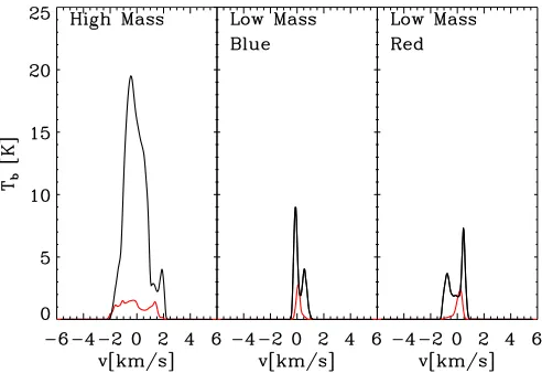
Figure 11.Illustration of the HCO+and N2H+(1–0) line profiles in high- and low-mass star-forming regions. The N2H+line has been multiplied by a factor of two to make it more visible and to allow a fair comparison, we chose a beam size of 0.01 pc throughout. The high-mass case corresponds to Region A viewed ati=90,φ=90. For the low-mass case we chose Core A fromPaper Iviewed ati=0,φ=0 (middle) andi=135,φ=0 (right), which have a blue and red asymmetry, respectively.
(A color version of this figure is available in the online journal.)
thick in the filament, rather than in the low-mass core, the core velocities will not contribute to the observed HCO+line profile. In the low-mass case only the dense core center contributes to the N2H+emission and so there is only a single component.
In the MSFRs the collapse motions extend over a larger region, so the lines are more likely to become optically thick in the collapsing medium surrounding the central core. However, the large velocity gradient across the region leads to little self-absorption and only a small offset between optically thick and thin components. MSFRs contain multiple dense cores, increasing the probability of detecting multiple components in optically thin lines. On the other hand, low-mass star-forming regions are usually not clustered, and therefore the profiles only contain a single component.
Figure 11 shows a comparison between the HCO+ and N2H+ (1–0) lines between a high-mass and low-mass core for illustrative purposes. For the high-mass case, we chose Region A viewed at an inclination and declination of 90 deg. For the low-mass case, we chose Core A fromPaper I. To allow a fair comparison, we chose a beam size of 0.01 pc for both cases, as this is more typical of the resolution in low-mass star-forming regions (e.g., Andr´e et al.2007). From many viewing angles inPaper I no clear blue asymmetry is seen, this corresponds to the case shown on the right (i = 135, φ = 0 inPaper I) where the HCO+(1–0) line is optically thick in the filament. In the middle panel, we show another viewing angle in which the HCO+ became optically thick in the low-mass core instead of the filament (i =0,φ =0 inPaper I). In this case the HCO+ (1–0) line is brighter due to the higher core densities relative to the filament, and the line has a blue asymmetry. The N2H+line has a single component. In the left panel we show the high-mass case, which has the brightest HCO+lines, and the profile peak is to the blueward side of the core rest velocity. The N2H+line clearly shows multiple components.
6. CONCLUSIONS
In this paper, we have carried out radiative transfer modeling of optically thin and thick line profiles arising purely from collapse motions in MSFRs. The underlying cloud model was
is caused by emission from dense substructure in the protocluster that, due to the sharp velocity gradient across the region, has a different velocity from the central core. The lines are broad, and the peak in emission does not necessarily correspond to the velocity at which the most massive star is forming.
3. Optically thick lines. The optically thick HCO+ (1–0) line shows only marginal blue asymmetries relative to the optically thin line peaks. The optically thick line peak is displaced by more than−0.5 km s−1in less than half of the calculated sightlines, which is small compared to the typical observed 2 km s−1 line width observed in such regions (Fuller et al. 2005). Moreover, there is rarely a central absorption dip due to the lack of a static self-absorbing envelope.
4. Time evolution. As the MSFR evolves its optically thick HCO+lines get brighter, and both optically thick and thin line profiles get broader.
5. Variation with beam.The line brightness increases and line width decreases as the FWHM of the beam is reduced. In our narrowest beam, the peak HCO+was more frequently to the blue side of the peak N2H+ emission. However, the N2H+profiles also more frequently contained multiple components in the narrowest beam. Such behavior would be an ideal prediction to test with ALMA in order to study the dynamics of massive star formation.
6. Higher-order transitions.Higher transitions of the optically thick HCO+ lines become increasingly Gaussian due to a growing fraction of the emission originating from a region with a large velocity gradient, where there is little self-absorption in the line. This suggests that the lower HCO+ transitions, namely (1–0) and (2–1) are better indicators of collapse for these regions.
7. Comparison to low-mass star formation.The optically thick lines of MSFRs are bright, and have large line widths. In low-mass cores, the profiles are less intense and have smaller line widths. The optically thin lines of MSFRs can have multiple peaks, due to the presence of numerous density enhancements along the line of sight. Alternatively, optically thin lines from low-mass protostars almost always have Gaussian profiles, since the ambient (filamentary) gas contributes little to the emission
We thank Amy Stutz for her work onPaper Ito which this paper is a sequel. R.J.S, R.S, and R.S.K. gratefully acknowledge support from the DFG via the SPP 1573 Physics of the ISM
REFERENCES
Aikawa, Y., Herbst, E., Roberts, H., & Caselli, P. 2005,ApJ,620, 330
Andr´e, P., Belloche, A., Motte, F., & Peretto, N. 2007,A&A,472, 519
Bate, M. R., Bonnell, I. A., & Price, N. M. 1995, MNRAS,277, 362
Bergin, E. A., Alves, J., Huard, T., & Lada, C. J. 2002,ApJL,570, L101
Beuther, H., Linz, H., Tackenberg, J., et al. 2013,A&A,553, A115
Beuther, H., Schilke, P., Menten, K. M., et al. 2002,ApJ,566, 945
Beuther, H., Sridharan, T. K., & Saito, M. 2005,ApJL,634, L185
Bonnell, I. A., & Bate, M. R. 2006,MNRAS,370, 488
Bonnell, I. A., Bate, M. R., & Vine, S. G. 2003,MNRAS,343, 413
Bonnell, I. A., Vine, S. G., & Bate, M. R. 2004,MNRAS,349, 735
Bontemps, S., Motte, F., Csengeri, T., & Schneider, N. 2010,A&A,524, A18
Cesaroni, R., Felli, M., Testi, L., Walmsley, C. M., & Olmi, L. 1997, A&A,
325, 725
Chen, X., Shen, Z., Li, J., Xu, Y., & He, J. 2010,ApJ,710, 150
Csengeri, T., Bontemps, S., Schneider, N., Motte, F., & Dib, S. 2011a,A&A,
527, A135
Csengeri, T., Bontemps, S., Schneider, N., et al. 2011b,ApJL,740, L5
Cyganowski, C. J., Whitney, B. A., Holden, E., et al. 2008,AJ,136, 2391
Dullemond, C. P. 2012, Astrophysics Source Code Library, 2015 Elmegreen, B. G. 2000,ApJ,530, 277
Evans, N. J., II 1999,ARA&A,37, 311
Fuller, G. A., Williams, S. J., & Sridharan, T. K. 2005,A&A,442, 949
Girichidis, P., Federrath, C., Banerjee, R., & Klessen, R. S. 2011,MNRAS,
413, 2741
Girichidis, P., Federrath, C., Banerjee, R., & Klessen, R. S. 2012,MNRAS,
420, 613
Jørgensen, J. K., Sch¨oier, F. L., & van Dishoeck, E. F. 2004,A&A,416, 603
Keto, E. 2007,ApJ,666, 976
Keto, E., & Rybicki, G. 2010,ApJ,716, 1315
Klaassen, P. D., & Wilson, C. D. 2008,ApJ,684, 1273
Klessen, R. S., & Burkert, A. 2000,ApJS,128, 287
Krumholz, M. R., Klein, R. I., McKee, C. F., Offner, S. S. R., & Cunningham, A. J. 2009,Sci,323, 754
Krumholz, M. R., & Tan, J. C. 2007,ApJ,654, 304
Longmore, S. N., Pillai, T., Keto, E., Zhang, Q., & Qiu, K. 2011,ApJ,726, 97
Mardones, D., Myers, P. C., Tafalla, M., et al. 1997,ApJ,489, 719
McKee, C. F., & Tan, J. C. 2003,ApJ,585, 850
Monaghan, J. J. 1992,ARA&A,30, 543
Motte, F., Bontemps, S., Schilke, P., et al. 2007,A&A,476, 1243
Myers, P. C. 2011,ApJ,735, 82
Myers, P. C., Mardones, D., Tafalla, M., Williams, J. P., & Wilner, D. J. 1996,ApJL,465, L133
Paron, S., Ortega, M. E., Petriella, A., et al. 2012,MNRAS,419, 2206
Peretto, N., Andr´e, P., & Belloche, A. 2006,A&A,445, 979
Peretto, N., Andr´e, P., K¨onyves, V., et al. 2012,A&A,541, A63
Peretto, N., Hennebelle, P., & Andr´e, P. 2007,A&A,464, 983
Peters, T., Longmore, S. N., & Dullemond, C. P. 2012,MNRAS,425, 2352
Rawlings, J. M. C., Redman, M. P., Keto, E., & Williams, D. A. 2004,MNRAS,
351, 1054
Rawlings, J. M. C., Taylor, S. D., & Williams, D. A. 2000,MNRAS,313, 461
Roberts, H., van der Tak, F. F. S., Fuller, G. A., Plume, R., & Bayet, E. 2011,A&A,525, A107
Robitaille, T. P., Whitney, B. A., Indebetouw, R., Wood, K., & Denzmore, P. 2006,ApJS,167, 256
Rod´on, J. A., Beuther, H., & Schilke, P. 2012,A&A,545, A51
Rygl, K. L. J., Wyrowski, F., Schuller, F., & Menten, K. M. 2013,A&A,
549, A5
Sanhueza, P., Jackson, J. M., Foster, J. B., et al. 2012,ApJ,756, 60
Schneider, N., Csengeri, T., Hennemann, M., et al. 2012,A&A,540, L11
Seifried, D., Banerjee, R., Klessen, R. S., Duffin, D., & Pudritz, R. E. 2011,MNRAS,417, 1054
Shetty, R., Glover, S. C., Dullemond, C. P., & Klessen, R. S. 2011a,MNRAS,
412, 1686
Shetty, R., Glover, S. C., Dullemond, C. P., et al. 2011b,MNRAS,415, 3253
Smith, R. J., Longmore, S., & Bonnell, I. 2009,MNRAS,400, 1775
Smith, R. J., Shetty, R., Stutz, A. M., & Klessen, R. S. 2012,ApJ,750, 64
Sobolev, V. V. 1957, SvA,1, 678
Sun, Y., & Gao, Y. 2009,MNRAS,392, 170
Tan, J. C., Krumholz, M. R., & McKee, C. F. 2006,ApJL,641, L121
Vasyunina, T., Linz, H., Henning, T., et al. 2011,A&A,527, A88
V´azquez-Semadeni, E., Kim, J., Shadmehri, M., & Ballesteros-Paredes, J. 2005,ApJ,618, 344
Walker, C. K., Narayanan, G., & Boss, A. P. 1994,ApJ,431, 767
Wu, J., & Evans, N. J., II 2003,ApJL,592, L79
Wu, Y., Henkel, C., Xue, R., Guan, X., & Miller, M. 2007,ApJL,669, L37