David Hunter
A Thesis Submitted for the Degree of PhD at the
University of St. Andrews
2009
Full metadata for this item is available in the St Andrews Digital Research Repository
at:
https://research-repository.st-andrews.ac.uk/
Please use this identifier to cite or link to this item: http://hdl.handle.net/10023/763
This item is protected by original copyright
three-dimensional Morphable Models
A thesis to be submitted to the
UNIVERSITY OF ST ANDREWS
for the degree of
DOCTOR OF PHILOSOPHY
by
David Hunter
School of Computer Science University of St Andrews
The ability to synthesise the effects of ageing in human faces has numerous uses from aid-ing the search for missaid-ing people to improvaid-ing recognition algorithms and aidaid-ing surgical planning.
The principal contribution of this thesis is a novel method for synthesising the visual ef-fects of facial ageing using a training set of three-dimensional scans to train a statistical ageing model. This data-base is constructed by fitting a statistical Face Model known as a Morphable Model to a set of two dimensional photographs of a set of subjects at different age points in their lives. We verify the effectiveness of this algorithm with both quantitative and psychological evaluation. Most ageing research has concentrated on building models using two-dimensional images. This has two major shortcomings, firstly some of the infor-mation related to shape change may be lost by the projection to two-dimensions; secondly the algorithms are very sensitive to even slight variations in pose and lighting. By using standard face-fitting methods to fit a statistical face model to the image we overcome these problems by reconstructing the lost shape information, and can use a model of physical rotations and light transfer to overcome the issues of pose and rotation. We show that the three-dimensional models captured by face-fitting offer an effective method of synthesising facial ageing.
has not been submitted in any previous application for a higher degree.
I was admitted as a research student in September 2003 and as a candidate for the degree of Doctor of Philosophy in September 2003; the higher study for which this is a record was carried out in the University of St Andrews between 2003 and 2008.
date signature of candidate
I hereby certify that the candidate has fulfilled the conditions of the Resolution and Regu-lations appropriate for the degree of Doctor of Philosophy in the University of St Andrews and that the candidate is qualified to submit this thesis in application for that degree.
date signature of supervisor
In submitting this thesis to the University of St Andrews we understand that we are giv-ing permission for it to be made available for use in accordance with the regulations of the University Library for the time being in force, subject to any copyright vested in the work not being affected thereby. We also understand that the title and the abstract will be published, and that a copy of the work may be made and supplied to anybona fidelibrary or research worker, that my thesis will be electronically accessible for personal or research use unless exempt by award of an embargo as requested below, and that the library has the right to migrate my thesis into new electronic forms as required to ensure continued access to the thesis. We have obtained any third-party copyright permissions that may be required in order to allow such access and migration, or have requested the appropriate embargo below.
The following is an agreed request by candidate and supervisor regarding the electronic publication of this thesis:
Access to Printed copy and electronic publication of thesis through the University of St Andrews.
No thesis can be written entirely single handedly, I am obligated to thank the following individuals.
First and foremost I wish express my gratitude to Dr. Bernard P. Tiddeman for his immense patience in supervising my research, for the invaluable advice and suggestions and for proof reading this thesis.
I am extremely grateful to Prof. D. Perrett of the School of Psychology at the University of St Andrews for providing the photographic data used in this thesis along with his advice on conducting perceptual experiments.
I would also like to thank Dr. Jingying Chen, Meng Yu and Zakariyya Bhayat for their help in gathering three-dimensional scans and putting dots on faces. Dr. Tim Storer for providing the LATEXclass files with wich this thesis is typeset. Norman, Andy, Jose and
Jim who keep the schools computers running, the school’s secretaries Gina and Joy and the many other people who keep the university functioning around us.
I also have to thank Richard, Sarah and Jonathan for their encouragement and friendship. Finally my parents whoes support and encouragement has never wavered.
this thesis
David W. Hunter and Bernard P. Tiddeman.
Towards individualized ageing functions for human face images.
In Theory and Practice of Computer Graphics, Bangor, United Kingdom, 2007. Euro-graphics Association.
Bernard P. Tiddeman., David W. Hunter, and Yu Meng. Fibre centred tensor faces.
InBritish Machine Vision Conference, volume 1, pages 449–458, 2007.
David W. Hunter and Bernard P. Tiddeman.
Visual ageing of human faces in three dimensions using morphable models and projection to latent structures.
InVISAPP 2009: Proceedings of the Third International Conference on Computer Vision Theory and Applications, Lisboa, Portugal, February 05-08, 2009, 2009.
List of Figures v
List of Tables vii
1 Introduction 3
1.1 System Overview . . . 5
1.2 Thesis Contribution . . . 6
1.3 Thesis Outline . . . 7
2 Literature Review 9 2.1 Early Methods . . . 10
2.2 Cardioidal Strain . . . 10
2.3 Overview of Statistical Representation of Faces . . . 11
2.4 Statistical Methods for Age Transformation . . . 12
2.5 Age Estimation . . . 18
2.6 Fine detail synthesis . . . 20
2.7 Summary . . . 21
3 Constructing a Three-Dimensional Morphable Model 23 3.1 Literature Review . . . 23
3.2 Constructing a Mesh Correspondence . . . 28
3.2.1 Iterative Closest Point alignment using multi-level free-form defor-mation . . . 28
3.2.2 Surface alignment using Parameterisation . . . 29
3.2.3 Results . . . 31
3.3 Principal Component Analysis . . . 32
3.4 Summary . . . 37
4 Fitting a Three Dimensional Morphable Model to an Image 39
4.0.1 Feature Extraction . . . 40
4.0.2 Alignment based methods . . . 40
4.1 Literature Review . . . 43
4.1.1 Active Appearance Models . . . 44
4.1.2 Fitting an Active Appearance Model to an image . . . 45
4.1.3 The Kanade Lucas Tomasi Algorithm . . . 46
4.1.4 Inverse KLT algorithm . . . 48
4.1.5 Projecting Out Appearance Variation . . . 49
4.2 Fitting a Morphable Model . . . 51
4.2.1 Extending the Inverse KLT algorithm to three-dimensional Mor-phable Models . . . 52
4.2.2 Feature Alignment . . . 53
4.2.3 Shape from Shading . . . 54
4.2.4 Error Functions . . . 54
4.3 Rendering . . . 56
4.3.1 Inverse Shape Projection . . . 57
4.3.2 Calculating lighting parameters . . . 60
4.4 Colour reconstruction . . . 60
4.4.1 Removing Lighting . . . 61
4.5 Implementation . . . 62
4.5.1 Point Alignemt . . . 64
4.5.2 The software . . . 70
4.6 Fitting Accuracy . . . 71
4.7 Summary . . . 74
5 Synthesising Facial Ageing 75 5.1 Ageing using Three Dimensional Morphable Models . . . 75
5.2 Ageing using Prototypes . . . 77
5.3 Individualized Linear Transform . . . 78
5.4 Partial Least Squares Regression . . . 81
5.5 Summary . . . 85
6.2 Perceptual Evaluation . . . 89
6.2.1 Identity Retention . . . 90
6.2.2 Perceived Age . . . 93
6.3 Summary . . . 97
7 Conclusions and Future Work 99 7.1 Summary . . . 99
7.2 Future improvements . . . 100
7.2.1 Final remarks . . . 102
1.1 System Overview . . . 7
3.1 The one-ring around vertex,vi . . . 27
3.2 Iterative Closest Point alignment . . . 29
3.3 Iterative Closest Point alignment algorithm . . . 30
3.4 Reconstructed mesh using surface parameterisation . . . 32
3.5 Reconstructed mesh using ICP . . . 33
3.6 Constructing a Morphable Model. . . 36
3.7 Examples of the shape changes associated with the first five Principal Com-ponents. . . 37
3.8 Examples of the colour changes associated with the first five Principal Components. . . 38
4.1 Calculating the parameter update for iterative face-fitting. . . 66
4.2 An example of a three-dimensional Morphable Model fitted to a face image. 69 4.3 Identity retention during face fitting stimulus . . . 72
5.1 Ageing using Prototypes. . . 79
5.2 Ageing using an Individualized Linear Transform. . . 80
5.3 The variance explained by the first 9latent vectors . . . 84
5.4 Examples of aged face images. . . 86
6.1 Identity retention during ageing stimulus . . . 91
6.2 Perceived age of age face model stimulus. . . 94 6.3 Distribution of age responses from human raters for rendered face models . 95
4.1 The Proportion Correct, d’ andχ2 for identification of fitted face models. . 73
5.1 Ageing dataset stratification . . . 77
6.1 Standard deviation weighted RMSE . . . 89
6.2 P.C. d’ andχ2 for retention of Identity. . . 93
6.3 Mean age for each method. . . 96
6.4 Mean age error for each method. . . 97
6.5 T-tests on means of absolute perceived age by ageing method. . . 97
4.1 Inverse Subtractive KLT algorithm . . . 65 5.1 PLS regression algorithm . . . 83 5.2 PLS ageing algorithm . . . 85
Introduction
Accurate prediction of how a person’s appearance will vary with age has a variety of ap-plications, such as helping in the search for missing persons, planning cosmetic surgery, as well as applications in the film industry and other visual arts. In this work we improve upon current two-dimensional methods by using a technique to fit a statistical face model, known as a Three Dimensional Morphable Model (3DMM) [15], to photographs of human faces. This aims to eliminate the problems associated with pose and lighting as well as ap-proximate the three-dimensional shape of the subject’s face. We use this data to investigate various multi-variate statistical methods which, we believe, will provide improved ageing functions by finding correlations between appearance and the way in which an individual ages.
Our method makes use of two databases for its calculations, one a set of 3D scans of individuals of a variety of ages, and the other a set of 2D images of individuals at multiple age points in their lives. The 3D scans are used to create a statistical model, containing the principal components or eigenfaces [85] of the scans. This model is used both to create 3D models from the 2D images and as a coordinate space with which to train the ageing function.
Two dimensional face models, by definition, store no information about the shape of the face in the depth plane, i.e. along an imaginary axis that points into the image. This results in a number of shortcomings in using these models for face analysis. The models are highly vulnerable to changes caused by rotations, perspective effects, or changes in the lighting conditions around the face being studied. As these effects are not related to ageing
it is important to eliminate them before attempting to train an ageing model, to avoid any spurious correlations. As an example, if most or all of the images taken of individuals in one age range were taken face on and most of the images of another age range were at an angle, the na¨ıve method would consider the changes in the image related to rotation to be the strongest correlates to ageing. Previous researchers have attempted to deal with the problem of pose in two-dimensions either by using a standardised image sets, or by using a two-dimensional linear transform to ‘de-rotate’ images. Standardised image sets where the pose and lighting of the subject can be controlled, are not always available and even small rotations can affect the results, so a method that eliminates the effects of rotations is preferable.
Lighting effects cause similar problems, although lighting can be described in a linear fashion in two-dimensions, either as a low frequency approximation [65] or as a point light source in image template alignment [74], these methods both rely on the absence of rotations and shadowing. Image normalisation can remove the effects of ambient lighting but are still prone to the effects of more directional lighting effects, such as diffuse lighting specular highlights and even area lighting. As a result, lighting effects have been found by some authors [71] to creep into ageing functions even when the images have been normalised.
A two-dimensional model can capture the shading changes related to three-dimensional shape change, provided the lighting is constant, however the lighting sources in our image-set are not constant and exhibit changes in lighting angle, composition and spread.
Using a three-dimensional model to describe the face can deal with these problems by syn-thesis. The effects of rotation, perspective changes, and lighting transfer can be described using physical modelling. As a result these effects can be used as independent parameters in the description of the fitted face model, and normalised in the age-model to remove their effects.
1.1
System Overview
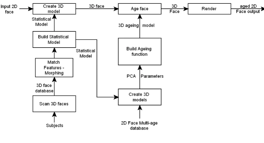
Figure 1.1 shows an overview of the face ageing system developed in this thesis. The system takes as input a two-dimensional image of a previously unseen individual. A new image is synthesized, based on the input and an ageing function, such that it looks like the same person aged by a specified amount. The system makes use of two databases for its calculations; one a set of three-dimensional scans of individuals of a variety of ages, sexes and lifestyles, and the other a set of two-dimensional images of individuals at multiple age points in their lives. The three-dimensional scans are used to create a generative statistical face model, containing the principal components or eigenfaces of the scans. This model is used both to create three-dimensional models from the two-dimensional images and as a coordinate space within which the ageing function is trained.
Three-dimensional Face Scans
Three-dimensional Models from Two-dimensional Images
3D scanners have been developed only recently, so collections of 3D scans of individuals at different ages are rare and incomplete. Waiting for individuals to age in order to rescan them is beyond the time frame of this project. Photography on the other hand has been in existence for over a century and photographs of individuals at different ages are relatively easily obtained. The proposed solution is to fit the 3D statistical model to the photographs and so obtain a 3D model of each face. A technique for obtaining these models has been developed by Blanz and Vetter [16] and has been successfully used in the field of face identification [15]. It has recently been applied by Scherbaum et al. to face ageing, this work was carried out concurrently to this thesis [72]. Scherbaum’s system differs from ours as they fit Morphable Models to parameterise three-dimensional scans rather than two-dimensional images. Park et al. also during the course of this thesis used a similar face-fitting method on two-dimensional images to train an ageing model [87], however they used a simple linear ageing method that did not attempt to take individual ageing patterns into account, or attempt to separate ageing related changes from other changes in the training-set. This system still offers the same advantages over 2D image analysis. Variations in pose can be accounted for using rotations and lighting effects, which can distort 2D image analysis, can help shape the 3D model.
Our 2D image dataset consists of 346 images of 43 different individuals taken at various age ranges. Infants between 0 and 1.5 years old, toddlers between 2 and 6 years old, mid child from 6 to 9, late child from 9 to 13, teenagers from 13 to 18 and students from 18 to 23. The images were gathered from images submitted by students of St. Andrews University and vary in quality, pose, lighting and completeness.
1.2
Thesis Contribution
In this thesis we make 4 main contributions;
• A complete system for ageing two-dimensional facial images using three-dimensional Morphable Models.
Figure 1.1: System Overview
individual in the image.
• A new statistical ageing method based on Projection to Latent Structures (PLS).
• A quantitative and perceptual evaluation of PLS based ageing and two other well known statistical ageing methods.
1.3
Thesis Outline
Literature Review
In the previous chapter we provided an overview of the full overview of both this thesis and the approach we will use to age a given face image. In this chapter we will describe the current state of the art in visual ageing of human face images, as well as providing an historical overview of its development. We will be concentrating particularly on computer modelling of facial ageing and the production of aged face images.
Previous research into ageing a face image has concentrated on transforming a two-dimensional image. At their core, these methods work by applying a shape and colour change to the input image often based on a statistical model. Early methods such as cardioidal strain, were non-statistical and relied on the similarity between mathematical functions and large scale biological changes [59, 60, 50, 88]. More resent researchers have used statistical modelling methods to derive a model from a set of training images [43, 71]. The primary variations in these methods have been the functions and methods used to train the model.
Much of the previous research can be broken down into two major categories; ageing sim-ulation and age estimation. Ageing simsim-ulation is the process of synthesising a face image such that it resembles an input face aged a specified number of years. Age estimation is the reverse of age simulation, using computer models to estimate the age of a person based on their physical appearance. Although this research concentrates on ageing simulation many of the ideas and principles behind age-estimation are still relevant. Also, some methods of automated age estimation have been used to perform ageing simulation, where image parameters are altered in order to match the recognised age to the desired age [43].
2.1
Early Methods
One of the earliest recorded techniques for face synthesis was invented by Galton in 1878. His method involved using multiple exposures of a single photographic plate to produce a composite image of a group of individuals. Alignment of individuals in the photographs proved difficult as faces come in a variety of different proportions. The resulting pho-tographs were blurred but features common throughout the group could be perceived [30]. Thompson [82] suggested the use of coordinate transforms for altering the shape of bio-logical organisms. Notably he showed that linear and non-linear transforms could be used to alter the profile of one species such that it approximates the profile of a different but related species.
2.2
Cardioidal Strain
2.3
Overview of Statistical Representation of Faces
Kirby and Sirovich [53] and Turk and Pentland [86] modelled the space of human faces using the Karhunen-Lo`eve theorem to build a set of basis vectors on a set of face images. The set of faces were centred by subtracting the average from each face image, and a set of eigenvectors, known as eigenfacescomputed from the matrix of covariants. The face images could be approximately reconstructed from a weighted linear combination of a lower dimensional subset of eigenfaces, and these coefficients then used for identification. The representation suffered from blurring effects as the features of the face were not in full alignment, meaning the edges of the same feature (e.g edge of the face) are not likely to be in the same sample area in multiple images. The result is a low frequency approximation. The algorithm was based on the intensity of the image samples only and so shape, view and illumination changes were only implicitly modelled and could not be separated from colour based variances. A more meaningful statistical face model can be constructed by bringing the faces into correspondence so that each pixel sample in the model corresponds to the same position on each face.
The three-dimensional morphable model [16] introduced by Blanz and Vetter is an ex-tension of the idea of using PCA to model variations in face shape and colour from two dimensional face images to three-dimensional models. As two-dimensional images are representations of a three-dimensional object they suffer from problems associated with pose and illumination. The projection of a simple rotation on to a two-dimensional im-age plane results in a warp that is neither linear nor injective. Linearity is a precondition for effective modelling with a linear basis such as PCA. The mappings are not injective (one-to-one) because points in three-dimensional space can appear and disappear as they become occluded and un-occluded. Illumination also poses a problem, although it has been shown empirically [65] that variations in lighting (including shadowing) can be modelled using a low-dimensional linear basis, this assumes no variation in the shape of the object, it also excludes shadowing. When either pose or shape is altered the relationship between illumination and image intensity becomes non-linear. Using a three-dimensional model these effects can be modelled physically. Like previous methods the morphable model de-scribes the shape and colour of the face separately as a weighted linear combination of basis vectors constructed from PCA plus the mean. Their implementation differed from AAMs in a number of respects; the shape is a mesh of three-dimensional points instead of two-dimensional points, the mesh contains many more vertices than an AAM and thus provides a dense representation of the face shape, the colour components are only defined on the vertex points and linearly interpolated between them. This was justified on the basis of the dense representation of the shape.
2.4
Statistical Methods for Age Transformation
Rather than develop a model of ageing independently, many researchers have used a set of training-data usually in the form of images, although some researchers have used three-dimensional scanning equipment [36] and Morphable Models [72, 87].
with the warp offsets defined as the shift between a feature point position on the face and the feature point’s position in the average. Rowland and Perrett [70] extended the method to perform facial transforms. The shape and colour differences between the averages of 20 young faces (males between 25 and 29) and 20 older faces (also males between 50 and 54 years) were used to create a simple transform. The differences were added to a target face using image warping to produce the appearance of ageing. They noted that both shape and colour changes separately produce an increase in perceived age, although the age difference produced by the combined shape and colour transform was significantly less than the 25 year age gap. They postulated that this was caused by the algorithm blurring out textural detail such as wrinkles. Importantly they showed that the transform maintains the identity of the person, thus the resulting image not only looks older but look like thesameperson older.
Burt and Perrett further investigated the process of ageing using these facial composites and transform algorithms [18]. They collected face images of 147 Caucasian males between 20 and 62 and divided the images into 7 sets each spanning 5 years. An average for each group was calculated along with a population average made by combining the groups. They found that the perceived age of the composite average of each group was consistent with the average perceived age of the individuals that made up the group, but noted that raters tended to underestimate the age of the composite images. This underestimation was greater in the older age groups than in the younger age groups. They concluded that the warping and blending process retained most of the age related information and suggested that the underestimation was due to a loss of textural detail in the blending process. In the same paper they described two different ageing transforms, one based on colour caricatures and another based on the vector difference between the oldest and the youngest groups. Colour caricatures were created by doubling the colour difference (in rgb space) between the average of the 50-54 age group and the population average. In the second transform they calculated the difference, in the shape and colour, between the oldest and the youngest age group. The shape and colour differences were then superimposed onto a target image. Experimental evaluation showed that both techniques produced a significant increase in the perceived age, although significantly less than the age difference between the original groups used to train the transform.
pa-rameterised using PCA. Their technique involved parameterising a set of two-dimensional face images using PCA, in a similar manner to AAMs [19], and then calculating ageing paths through the parameterised space. They delineated key features (eyes, ears, chin etc.) on a set of photographs. A shape average could then be computed by averaging the posi-tions of the feature points. Intensity information was also sampled from within the facial region. The feature points were concatenated into a single shape-vector. The intensity in-formation of the shape-normalised faces were also concatenated into a single colour-vector. Principal Component Analysis was performed on the covariance matrix of the shape-vector deviations were used to find the main axis of variations from the mean, leading to a com-pact parametric description of the shape of each face. PCA was also performed on the colour-vectors. This method gave them a set of low-dimensional parameters that can be used to both describe a set of faces and also by manipulating the parameters to describe new faces.
Given a set of parameterised faces of a set of individuals at various age points they where able to generate a series of age functions through the PCA face space that describe ageing. Using a genetic algorithm they were able to find polynomial curves, of degree 1,2 and 3, that related the parameters of the face model to the age of the face. This they called aglobal ageing functionas it assumed that all faces age in the same manner. These functions were used to estimate the ages of face images. They compared the accuracy of the age estimation produced by the polynomials to the known age of the individual. They found that both the quadratic and cubic polynomials offered a significant improvement over the linear, degree one, age functions. However the improvement offered by the cubic polynomial over the quadratic was slight, and so they chose the quadratic polynomial, as it was the simpler of the two.
gener-ate individualised ageing function for an unseen individual as a weighted sum of the ageing functions for similar individuals in the dataset. The similarity between two faces was esti-mated using the probability distribution generated from the construction of the PCA model. They also gathered lifestyle information about the individuals in the dataset, information such as gender, socio-economic factors, weather exposure etc, by asking those volunteering facial images to fill in questionnaires. The lifestyle information was vectorised and scaled such that the total variance in lifestyle information equalled the total variance of the facial parameters. In this way a new ageing function can be generated by weighting the ageing functions in the dataset by the combined appearance-lifestyle probabilities. This produced a higher correlation co-efficient of 0.72 suggesting that lifestyle has a significant impact on the visual effects of ageing, thus they were able to confirm known results from (biology, medicine references). By comparing the estimated ages of the face images to the known ages using a leave-one-out method they were able to show that individualised age models produce a more accurate estimation than global ageing functions. This was the case for both appearance based weighting and combined lifestyle appearance weighting. However this method relies on the existence of similar faces in the training set, otherwise the age function tends towards the global age function, as Lanitis et al. showed by attempting to estimate the ages of faces from a different ethnic group than that used to train the age model.
Their work also covered the area of synthesising facial ageing, generating the aged face images using the inverse of the polynomial functions used in age estimation. The results of the age synthesis where evaluated both quantitatively and perceptually. The parameters of the aged faces were compared to the parameters of a face image of the same individual at the target age using the Mahalanobis distance. The rendered face image were also shown to a set of human raters, who were asked to judge whether the synthesised image looked older than the original un-aged image, and whether the rendered image was more similar to the target individual than the original. They concluded from both the quantitative and perceptual results that both global and individual ageing functions produced suitably aged individuals, but that the individualised method was the superior method.
subjectively by human observers and then defined in the face space as the sum of score-weighted face parameters. Weighted multiples of these vectors were then used to alter the pose and expression so that they became uniform. This method approximates the rotation of a three-dimensional object on a two-dimensional plane by a linear method, this is a rea-sonable approximation provided the angles between the face pose and the normalized pose are small. In the event that the angle is large, this approximation becomes less accurate. Even in small rotations parts of the face that are occluded become visible, the textures are unknown and must be approximated, Scandrett at al. achieved this by reflecting the nor-malized image about its vertical axis. Like other 2D ageing methodologies Scandrett found that lighting variations reduced clustering of face-parameters of around the same age and thus the quality of aged textures. This effect was particularly pronounced with trajectories derived from an individual’s history using fewer face samples resulting in less smoothing of errors.
Each of the trajectories were designed to extract different factors that effect ageing, such as personal history, sex, how parents aged etc. The trajectories where defined as the sum of the face parameters centred on the group mean weighted by the mean shifted age of each face. Face images were aged by altering their parameters in the direction of one or more combined ageing trajectories until the target age is reached.
As males and female are known to age in different ways, separate ageing trajectories were produced for male and female in each group. An input face was then compared to these ageing trajectories to determine the comparative influence of the male and female trajecto-ries using a ratio of distances from the face to each trajectory.
The results were analysed using the root-mean-squared error, both on the shape vertices and per pixel, between the resulting face image and a known ground truth image of the individual at the target age. The faces having been converted to grey-scale and normalized to have a mean intensity of zero and standard deviation of one, in order to remove some of the effects of lighting on the results. They found that in general the root-mean squared shape and texture errors were lower when compared to a the ground truth image than with other images in the target age set, and concluded that the ageing methods both aged the individuals appropriately and retained identity through the transform. They found that the most accurate method of ageing varied between individuals and so could not conclude which method had the best performance.
Scherbaum el al. [72] fitted a three-dimensional morphable model to database of laser scanned cylindrical depth-maps. They used a database of 200 adult images and 238 teenagers. The later group ranged in age from 96 months to 191 months. In order to improve the res-olution of the face texture map, they reconstructed the textures from three photographs taken at three separate angles. They used the parameters of the model and the age of the subject to train a Support Vector Regression model. The S.V.R. formed a mapping from the high dimensional parameter space of the model to the<space of the subjects age. This was used to estimate the age of the subject once the parameters of the morphable model have been found. A new face model could be synthesized from a given set of parameters by ‘stepping’ through the curved SVR space using a fourth order Runge-Kutta algorithm, using the parameters and an estimated age as the starting point.
They didn’t use multiple time-space images of the same individual in building the model, their claim to individualization is the observation that, based on the mean angles between the support vector gradients, the SVR produced different ageing trajectories for different individuals and could therefore be said to be individualized. While this is true, the variation is derived from a large number of single ‘snapshots,’ i.e. it describes the variations within a population. It may not necessarily capture the variations due to ageing in a particular individual.
target age given the current set.
Park et al. [87] performed a similar experiment to ours fitting a three-dimensional Mor-phable Model to a set of delineated faces using point data. Ageing was performed by cal-culating a set of weights between an input face and exemplar faces in the same age group. These weights are then used to build an aged face as a weighted sum of the corresponding faces at the target age. The results were compared using Cumulative Match Characteristic curves to other ageing methods and reported similar results to other methods. They ob-served that shape modelling in three-dimensions gave improved performance in pose and lighting compensation. Their method differs from ours in that they only fit to the delineated point data rather, whereas our method used both point and pixel information as detailed in the following chapters 4.5.1.
2.5
Age Estimation
Age Classification is the conceptual opposite of ageing synthesis. the age of the face is estimated from an image rather than synthesizing a change resulting from age.
Kwon et al. [41] used the ratio between facial features, the nose, eyes and mouth, as well as wrinkle analysis. If wrinkles were found and ratios indicated an adult face, the image was marked as a senior adult. An image with no wrinkles and a baby-like ratio between features was marked as a baby. Otherwise the image was marked as an adult. This idea was expanded upon by Horng et al [89], who used a three phase method; feature location, extraction and classification. Two geometric features; the ratio distances between eyes and nose and between nose mouth, detected using a Sobel edge detector, and three wrinkle regions were detected. A Sobel edge detector was used to classify wrinkle density, with density defined as edgesarea. The age was classified to one of four age groups using back propagation neural networks. Kalamani and Balasubramanie used a fuzzy neural net to account for uncertainty in the classification model. Images were classified according to a
degree of inclusion [39].
maps. They also introduced three new types of classifier based on the training method. Firstly a classifier they calledage-specificwhere the faces were grouped into strata accord-ing to age prior to trainaccord-ing, where the classifier was only expected to place the input face into the relevant strata. Secondly a classifier they calledappearance-specificthat grouped images according to observation [43] of the relationship between appearance and ageing patterns, divided the individuals into groups of faces that appeared similar or aged in a similar manor. Thirdly a combination of the two. The methods were evaluated and com-pared using two-fold cross validation with the mean average error in years, between the classification result and the known ground truth. The new classifiers improved accuracy, and offered greater improvements when combined. They used perceptual evaluation of the training images with 20 human raters to gauge the accuracy of human age perception. The raters were shown the whole image, including details such as hair line. This is known to affect how humans rate an individual’s age. Human raters out performed the computers albeit on a much reduced number of test images.
2.6
Fine detail synthesis
Many of the statistical methods used lost textural detail such as wrinkles, a few researchers developed methods that attempted to create appropriate textural detail in aged images. Tid-deman et al. used a wavelet transform [83] and Markov Models [84] , Hussein used Bidirectional Reflectance Distribution Functions [35] and Gandhi used Gaussian filters [31]. These methods work by attempting to replace or adjust the high-frequency compo-nents of the image to match the high frequency compocompo-nents of a prototype at the target age.
Hussein [35] synthesised wrinkles by attempting to align the surface normals of two faces, an older and a younger using the relationship between pixel intensity and surface orienta-tion. Under the assumption that the two surfaces shown in the image are co-incident and under the same lighting conditions, surface details such as wrinkles would become the pri-mary changes in intensity. They used the ratio of the two images smoothed with a Gaussian filter multiplied with one of the images so that the fine detail of the other was applied to it. Their method suffered from two main drawbacks, firstly it could not be used under varying lighting techniques, secondly the age was defined from only one image and thus would not in general produce a convincing ageing result for an arbitrary individual.
Gandhi [31] used an Image Based Surface Detail Transfer [47] procedure to map the high-frequency information from an older prototype to a younger, and visa-versa using a Gaus-sian convolution as a low pass filter. The idea here being to take the high-frequency details of the input image and replace them with the target’s. The Gaussian convolution producing two images, one the smoothed original containing the low-frequency large scale detail and the other, the result of applying a standard boost filter, containing the high-frequency fine scale details. An aged image was synthesised by combining the high-frequency of a proto-type with the low-frequency of the image. Varying the width of the kernel would vary the size of details captured and thus the perceived age of the person. The prototypes at each age were created by averaging all the images in an age group. Smoothing problems were avoided by combining the high-frequency parts of the training images with the combined average to retain fine detail.
The edge magnitudes were then smoothed with a B-spline filter to give a measure of edge strength about a particular point in each sub-band. Prototypes at each age were generated using the technique of Benson and Perret [13] and the wavelets were then amplified locally to match the mean of the set. The values of the input wavelet images were modified to more closely match those of the target prototype. These were tested perceptually and found to reduce the gap between the perceived age of the image and the intended age. They then extended their method using Markov Random Fields [24]. An individual was aged using the prototyping method of Burt and Perret described above [18]. Detail was added to the resulting face by decomposing the image into a wavelet pyramid and scanning across the sub-bands using the MRF model to choose wavelet coefficients that match the cumulative probability of the input values. They found that human raters found the resulting image more closely matched the target age of the older group than either the Wavelet method on its own or the prototyping method, it also succeeded in the rejuvenating test where wavelets failed. They also found that humans rated the images more realistic than those generated using Wavelets alone [84].
2.7
Summary
In this chapter previous work in the area of facial age estimation and ageing simulation has been reviewed. In the course of this work we identified several desirable properties for an improved face ageing method, most of which have been included in previous methods, but have not previously been combined in a single implementation, these include:
• The use of 3D models to properly model (and allow removal of) the effects of lighting and out of plane rotations.
• The use of training data that includes within subject age variation to include a degree of individuality in the ageing model.
• The use of modern machine learning and statistical tools for learning and applying the ageing changes.
Constructing a Three-Dimensional
Morphable Model
In the previous chapter we provided a detailed overview of current methods in synthesising ageing in human face images. We also identified key properties of these algorithms that are desirable in an improved ageing model. In particular the use of a three-dimensional statistical model to describe the set of human face models. In this chapter, we describe a statistical face model that can be used to parameterise an input face. We also describe how this model can be used to render an image of a synthesised face model under a given set of pose and lighting conditions. Finally, we describe how the textural properties of a face can be reconstructed from partial data.
3.1
Literature Review
The face models produced by the three-dimensional capture system we are using are in the form of a triangular mesh, defined as a set of points (vertices) and a set of edges linking these vertices to form triangles. However each scanned face model is independently pro-duced and as such has an irregular structure. The meshes all have differing edge topologies, that is different edge structures linking vertices in the mesh. Also each point on the surface of a particular mesh has no predefined matching point on the surface of any of the other face models produced by the scanner. In order to build a statistical model these sets of face
models must be brought into a meaningful correspondence across subjects. The data from the scanner can also contain errors, e.g. noise and missing data, which manifests itself as holes on the face. Noise can be dealt with using a smoothing operator, but holes are more serious, requiring detection and interpolation.
A number of algorithms have been developed in the area of registration, tailored to tackle specific problems, such as point alignment, line and edge registration, and surface regis-tration. We wish to look specifically at the area of registering a set of three-dimensional triangular meshes of irregular edge topology such that we can generate of set of meshes are of corresponding edge topology but with varying surface shapes. Our meshes contain holes both around the edges of the mesh and internally that need to be identified and filled in a meaningful manner.
We define the face model as a tuple containing a shape description and a texture-map. The shape is described using a triangle mesh,M= (V,E). V is a set of verticesvi ∈ R3,ti ∈
T2,i = 1, . . . , n, where vi describes the position of the ith vertex in three-dimensional
space andti describes the location in texture spaceT2, i.e. ti = (ui, vi), ui, vi ∈[0,1]that holds theith vertices’ colour.E is a set of edges connecting the vertices,V. We have a set of three-dimensional meshesMj, j = 1, . . . , mthat we wish to use to build a statistical face model. We need a method that can construct a set of meshes, M0
i = (V0i,E), which describe surfaces as close as possible to the shape of their corresponding meshMbut have a common edge topology,E.
Iterative Closest Point alignment
The Iterative Closest Point alignment (ICP) method can be used to match multiple scans of human bodies to a common template [4, 5]. A set of correspondences between the vertices of the template mesh and the surface of the template mesh is found by locating the nearest point to each vertex on the target mesh. Obviously this assumes that the meshes are already in close proximity. A deformation field is then found that matches the displacements of each set of correspondences. The template mesh is updated with this deformation field and a new set of closest point correspondences generated. These steps are repeated iteratively until the meshes are sufficiently aligned. Not all the possible correspondences between template and surface are valid, and so a regulatory term is typically added. Besl and McKay defined the field globally [14], Feldmar and Ayache [26] defined the affine transforms locally over a spherical region. Allan et al. [4] and Amberg et al. [5] defined the field as an affine transform per vertex, this transform is not sufficiently constrained by a single correspondence and so used a regularising term to constrain the result. The closest point is generally found either by searching along the normal, [3, 33] or by finding the closest point in any direction [14, 26, 4, 5]. A search along the normal has an advantage over the closest point in that the space of searches matches the curve of the surface, however on surfaces exhibiting rapid changes in direction the search can potentially cross before finding a match. A regularisation term ensures a smooth deformation field between the two surfaces, Feldmar and Ayache [26] used the two principal curvatures of the surfaces to drive the matching towards similar features. Allen et al [4] used the sum of the Frobenius norm between affine transforms defined for adjacent vertices on the template mesh as part of the minimisation to weight the fitting towards smoothly varying deformations fields. Amberg et al. modified this metric to allow a weighting between the rotational and skew parts of the deformation at each vertex [5].
Remeshing
ICP algorithms assume that even if the vertices and topology of meshes are not in any sort of correspondence, the surfaces of the meshes are already closely aligned. If, however the surfaces are not in close correspondence ICP can produce some spurious results. Methods based on completely reconstructing meshes can find correspondences between surfaces that are not already in close proximity.
Instead of fitting a template mesh to a set of meshes, a new mesh can be constructed from the input meshes in a consistent manner so that the resulting meshes are in one-to-one correspondence. This method is known as remeshing. The method relies on the fact that a well defined triangle mesh forms a surface, a mapping can then be generated to map this surface from three-dimensional space to a two-dimensional space, a new mesh can then be generated by sampling at regular intervals within this two dimensional space and mapping back into the original three-dimensional space. The method of generating this mapping is known as parameterisation and was first described by Tutte [79]. Here I outline the method described by Floater [27] using mean-value coordinates [28].
Given a triangular meshM= (V,E)we desire to create a one-to-one mappingu :<3 →
<2from the 3D mesh surface to a plane. As the surface is three-dimensional, the resulting mapping will distort the mesh, a mapping that best preserves the angles and distances between the vertices when mapped onto the two-dimensional space is desirable.
The position of a vertex in the two-dimensional plane is defined as a weighted sum of the positions of its neighbours in the edge graph E. The weights are derived from the three-dimensional structure of the mesh, and it’s these weights, defined along the edges,
E, that help preserve the relative positions and angle of the vertices when mapping to a two-dimensional plane. A vertexvi ∈ R3 and its corresponding vertex on the plane, ui ∈
R2 form the mapping on the vertex. Between the vertices the mapping is defined using
defined the position on the plane of theithvertex as, ui−
J
X
j=1
λi,juj = K
X
k=1
λi,kbk, i= 1, . . . , n (3.1) where J and K are the number of internal and external vertices respectively. Here λi,j defines the weight along the edge i, j in E. If edge (i, j) is not in E then λi,j = 0. The weight is defined in such a way as to preserve the structure of the mesh, minimise stretching and preserve the angles between vertices.
λi,j =
wj
P
k∈Ωwk
, wj =
tan(αj/2) +tan(αj−1/2)
||vi−vj||
(3.2)
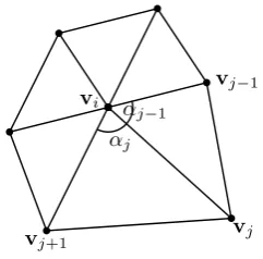
where k ∈ Ω is the one-ring of neighbouring vertices to i, that is, all vertices directly connected to the ith vertex by and an edge. The middle component of the equation is a normalisation term ensuring that Pk
j=1λi,j = 1 for all i. The final part of the equation defines an un-normalised weight in terms of the angles about the vertexialong both sides of the edge(i, j)and the length of the edge(i, j), see figure 3.1.
The two-dimensional positionsuiare found by solving the linear equation defined by equa-tion (3.1).
A more detailed survey of parameterisation techniques for three-dimensional meshes can be found in [29].
vi
vj vj
−1
vj+1 αj
αj
[image:46.595.260.381.476.595.2]−1
Figure 3.1: The triangles of the one-ring around vertexvi, illustrating the construction of the weight λi,j along the edge(i, j). The weight is computed as a function of angles αj,
αj−1 about the edge and the inverse of its length.
into a set of triangular patches using a common high level topology. Each patch was sep-arately parameterised by fixing the boundary vertices to a triangle in two dimensions and generating a mapping using Floaters parameterisation method (described above) [62].
The method of parameterisation is better able to cope with matching surfaces with poor initial correspondence. However, due to the parameterisation method only applying to internal vertices, it is unable to deal effectively with holes in the mesh.
3.2
Constructing a Mesh Correspondence
Before a statistical model can be built, the meshes must be brought into a one-to-one corre-spondence. In order to do this we define a template meshS = (V,E)and adapt this mesh to the input meshes, so that all the meshes share the same topological structure,E.
We implemented two methods for building a mesh correspondence. The first is based on the method by Praun et al. [62] using parameterisation and the second is based on ICP which is described below.
3.2.1
Iterative Closest Point alignment using multi-level free-form
de-formation
We adapt a reference face model to each subject’s face as outlined in figure 3.3. The two surfaces, the subject and the reference are brought into alignment by translation to a common mean and removing rotational variance between the two meshes. The translation to the mean is found by making the centre of mass of the point sets equal. The meshes are scaled by normalising the deviation from the mean and the required rotation found using SVD on the cross-covariances between pairs of meshes.
S
T
v1
v2
v3
v4
v5
v6 v01
v02
v03
v04
[image:48.595.157.539.77.351.2]v05 v05
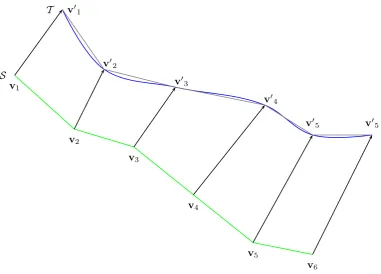
Figure 3.2: Surface S is matched to surface T using Iterative Closest Point alignment. Each vertexviis matched to a vertexv0iby searching along the surface normal.
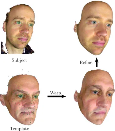
[45, 46]. We have implemented the MFFD warping using a space and search efficient oc-tree data structure. Once the face meshes are in approximate alignment correspondences are found using a standard ray-tracing algorithm. Rays are traced out of the reference mesh from each vertex in both directions along the surface normal and the first intersection (within a maximum radius) with the target face is found using an octree ray-tracing method (see figure 3.2). Not all vertices will find a target, and so these displacements are interpo-lated (again using MFFDs) across the reference mesh. This brings the reference mesh into good alignment with the subject.
3.2.2
Surface alignment using Parameterisation
Subject
Template
Warp
[image:49.595.66.442.132.563.2]Refine
ui ∈ R2 is found on the plane, such that the mesh is ‘flattened’ on to the surface of the plane in a manner that best preserves the angles between edges of the mesh and the lengths of edges (see section 3.1). Each position within a triangle on the surface of the mesh can be mapped onto the plane by finding its associated triangle in the flattened mesh and de-termining its position in this mesh using the method of barycentres. This produces a set of flattened meshes. These meshes can be brought into correspondence using the delineated points, for each delineated point on the surface of the mesh the corresponding point on the plane as found using the mapping,w. This produces a set of templates in two-dimensions for each input face. An average of these templates was found using Generalised Procrustes alignment [25] and warping between each template and the average generated using Thin Plate Splines (TPS). The application of this warp to flattened meshes brings them into cor-respondence on the plane. A new mesh can be generated by regularly sampling along a predefined grid on the plane in the area of the warped mesh. Using the TPS warp on the vertices of the mesh is possible but is not easily defined within the triangles of the mesh, instead we use an inverse warp on the sample points of the regular grid this allows us to sample from the triangles as if they were warped. For each sample point in the regular grid the triangle of the flattened mesh containing it is located and its corresponding point on the surface of the three-dimensional mesh found by inverting the mapping,w. If no triangle is found containing the sampling point the sample point is marked as missing. A new mesh is constructed by triangulating the located sample points in a ‘chess-board’ pattern with two triangles being formed in each quad.
3.2.3
Results
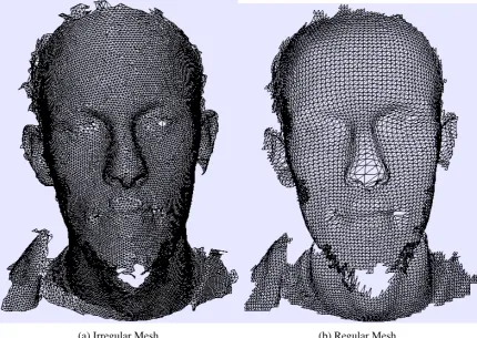
(a) Irregular Mesh (b) Regular Mesh
Figure 3.4: ‘Before and after’ view of a reconstructed mesh. The left hand image shows a ‘wire-frame’ view of a mesh as produced by the scanner. The irregular structure of the mesh is clearly visible as are the holes. The right hand image shows a reconstructed mesh, the regular grid pattern is visible as are the un-patched holes in the mesh.
The average of a set of 106 face models produced by the three-dimensional scanner was produced by aligning these meshes to a ‘reference mesh’ using the ICP fitting method. These aligned models were used to build a face model as described in the next section. The mean of the face models can be found in figure 3.5.
3.3
Principal Component Analysis
(a) Average Mesh (b) Front View (c) Profile View
Figure 3.5: Average of a set of face meshes constructed using Iterative Closest Point align-ment. Left is a wire-frame image of the full average mesh. Centre and right is are a face-on and profile rendering of the mean shape and colour of the set of face meshes. The centre and right meshes have been clipped to the facial area.
and arranges these according to their likelihood.
Principal Component Analysis (PCA) is a dimensionality reduction and decorrelation tech-nique. It finds a set of orthogonal basis vectors that span the data such that the covariance matrix is diagonal. In other words the data is linearly decorrelated. The first vector of the basis, the first principle component, is parallel to the direction of greatest variance in the data. The second vector is parallel to the direction of the next greatest variance and so on. Here we describe explicitly the method we used to calculate PCA on the shape data, the same method is also applied to texture data. This is a standard method [63]. In order to build a statistical model, the face shapes were first brought into a one-to-one correspon-dence between each face (see section 3.2). The three-dimensional positions of the vertices of the mesh were then concatenated to form a shape-vector,
s= (X1, Y1, Z1, X2, Y2, Z2,· · · , Xn, Yn, Zn)T, (3.3) wherenis the number of vertex points in the face models. With a set ofmexemplar shape-vectorssiwherei∈1. . . mwas centred by subtracting the meanˆsand arranged in a matrix
D, the eigenvectors and eigenvalues of its covariance matrix C were computed using the Jacobi Method [63] onC.
from between the mean and the set of shapes under a Euclidean similarity (scale, translation and rotation) transformation. Here we define the matrix R ∈ SO(3) to be the rotation matrix, a vector describing translations, t ∈ <3, and a scale κ ∈ <. Given two sets of vertex pointspandqwe alignqwithpby,
p =κqR+ 1mtT +E (3.4)
where E is an m ×3 error matrix and 1m is a 1× m vector of 1s. In two dimensions this can be solved by converting the two-dimensional points into a set of points in complex space,(x+yı) and finding the mean as the principal eigenvector of the complex covariance matrix, this is known as the full Procrustes algorithm [25]. In three dimensions it was solved in an iterative manner. First we calculated the translation,tby making the centre of mass of the point sets equal.
ˆ p= 1
n
n
X
i=1
pi. (3.5)
wherepi is the ith point in the vertex point set p. Similarly for q. The scale factor was chosen such that the l2-norm of pˆ and ˆqare both equal to 1. The mean centred and unit scaled points sets are denotedp˙ andq. The rotation matrix˙ Rwas found using SVD on the cross-covariance matrix,
˙
pTq˙ =VΛUT (3.6)
V andU form a set of orthonormal basis vectors inSO(3). R was updated asR = U VT withκ=trace(Λ)
The covariance matrix of residuals from the shape mean, C, can be calculated using the outer product of the matrixDwith itself,
C= 1
mDD
T (3.7)
However, this matrix is huge, having a width and height of the length of the vector s. We used a more practical alternative making use of the fact that the non-zero eigenvalues of m1DTD are identical to the non-zero eigenvalues of 1
mDD
T, using the inner product, 1
mD
The eigenvectors of the covariance matrix,C, are rearranged in descending order of their associated eigenvalues. These rearranged eigenvectors form the columns of the matrixU, and the eigenvalues form the vectord. We denote theithcolumn of the matrixUasu
i. Here the vectorsuiare simply the reordered eigenvectors denotedyi above. These eigenvectors form a linear basis that exactly spans the space of the faces used to build the PCA model. The eigenvectorsdare related to the variance of the distribution asσi2 = di
m wheredi is the
ith eigenvalue in d andσ
i is the standard deviation in the direction of the corresponding eigenvectorsi.
A significant benefit of PCA is that we can perform a dimensionality reduction on the face-space. We selected a subset of vectors of U to form a basis from which each exemplar face can be approximately reconstructed and new faces synthesised. As the columns ofU
had already been reordered we could form a basis in l dimensions simply by taking the first l column vectors inU. We denote this basis Sl(×l)n = [y1,y2, . . . , yl]. This optimally minimises the residual error under thel2−norm. We wished to find the minimal value of
l such that an acceptable amount of the variance in the dataDis explained byS(l). If we define the cumulative energy asgi =
Pl i=1di
Pm
i=1di, i.e. the cumulative sum of the singular values up tolweighted by the total sum. lis therefore the minimum value such thatgl≥, where
is the amount of variance the model is required to explain . The firstlvectors are known as the principal components.
We were therefore able to define a new shape descriptor as a linear combination of principal components:
s=ˆs+ l
X
i=1
αiyi (3.8)
The new descriptor spans the space of the shape exemplars up to an accuracy of gl. The probability distribution of the shape descriptor is:
p(s)∼e−
1 2
P
i α2i
σs,i (3.9)
The range of fitting is thus constrained in a maximum-likelihood sense to those most likely to correspond to the identity of the face shown in a particular image.
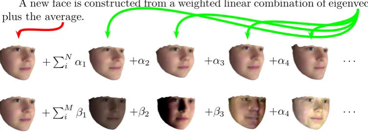
A new face is constructed from a weighted linear combination of eigenvectors plus the average.
+PNi α1 +α2 +α3 +α4 . . .
+PMi β1 +β2 +β3 +α4 . . .
[image:55.595.58.436.87.225.2]Each face can then be described as (α1, α2, . . . αN, β1, β2, . . . , βM).
Figure 3.6: Constructing a Morphable Model.
was defined as a two-dimensional image mapped onto the surface of the model using a set of discrete texture coordinates defined for each vertex and linear interpolation to define the mapping within the triangles of the mesh. The colour-maps for each of the face models were registered and the discrete texture coordinates computed during the morphing process.
The pixel values of each input image were concatenated as,
t= (R1, G1, B1, R2, B2, G2,· · · , Ro, Go, Bo)T (3.10) and PCA performed, by the same method as for the shape components, to produce,
t=ˆt+ l
X
i=1
βiti (3.11)
whereti is theitheigenvector of a covariance matrix of the registered colour-maps and β is a set of colour components.
As before the space of the colour model is reduced to the firstl principal component vec-tors. A new face colour can be constructed as a linear combination of the principal compo-nents weighted with a set of parametersβ. The probability distribution of the new colour descriptor is,
p(t)∼e−
1 2
P
i βi2
σt,i (3.12)
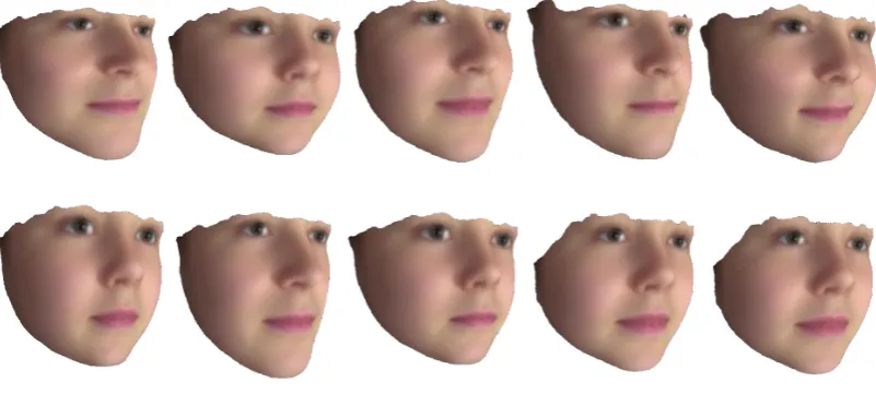
Figure 3.7: Examples of the shape changes associated with the first five Principal Compo-nents. Each of the images shows a model rendered with the specified component increased by an arbitrary amount in the top row and decreased by same amount in the bottom row.
shape and colour is defined as,
p(s,t) =p(s).p(t)∼e−
1 2
P
i α2i σs,i.e−
1 2
P
i β2i
σt,i (3.13)
Figures 3.7 and 3.8 show the shape and colour changes associated with the first five Prin-cipal Components of the face-set. The first few eigenvectors of the colour prinPrin-cipal com-ponents clearly contain significant lighting information, this is due to the variable lighting condition under which the faces were scanned and the texture maps produced. This means that some of the model parameters may contain unwanted lighting information in later stages, such as fitting or ageing.
3.4
Summary
Figure 3.8: Examples of the colour changes associated with the first five Principal Compo-nents. Each of the images shows a model rendered with the specified component increased by an arbitrary amount in the top row and decreased by same amount in the bottom row.
• The ability to generate a set of meaningful one-to-one correspondences.
• A technique to fill holes in the mesh.
Fitting a Three Dimensional Morphable
Model to an Image
In our literature review of current methods for synthesising face ageing, chapter 2, we identified an individualised ageing model as superior in accuracy to a global ageing model. This requires a set of three-dimensional face models of the same individual at multiple age points. At the time of writing such data-set were unavailable, due to the relative nov-elty of three-dimensional scanning equipment. A suitable set of three-dimensional face models can be generated by extracting three-dimensional information from a set of two-dimensional image. Two-two-dimensional image-sets being much more readily available. This extraction is achieved by fitting a three-dimensional Morphable Model to the images, by minimising the error between the rendered Morphable Model and the target image.
In this chapter, we outline the algorithms that have been developed for fitting a three-dimensional Morphable Model to a two-three-dimensional image. From these, we select a suit-able algorithm, describe our implementation, and present some results of our implemen-tation. For the face-fitting method to be useful in developing ageing models it must be able to extract an accurate three-dimensional representation of the individual depicted in the image. Towards the end of this chapter we will describe an experiment to evaluate how well the three-dimensional models represent the individual in the image by determining if a set of human observers can recognize the individual from their rendered model.
The face models extracted by this process are used to train a statistical ageing model in
order to synthesis the aged appearance of a face.
We begin by describing some of the most commonly used algorithms for fitting Active Appearance Models (AAM), the two-dimensional analog of three-dimensional Morphable Models (3DMM) and discuss their application to fitting 3DMMs. Then we outline current methods devised specifically for fitting 3DMMS to a two-dimensional image.
4.0.1
Feature Extraction
A description of the shape and colour of a human face in an image can be extracted by aligning the statistical face model with the image in such a way that the error between the rendered face model and the image is minimised. This is normally achieved by varying the parameters of the face descriptor in such a way that a cost function is minimised. Although the parameters of the Morphable Model are defined as a linear combination of basis vectors, the fitting operation is not linear. In general, the intensity of a pixel is not related to its position in the image plane, as a result there does not exist a linear relation between shape changes in the face model and the resulting change in the image intensity of a particular sample point. Other sources of non-linearity result from the three-dimensional nature of the face model, rotations in particular result in occlusions and in changes in relative position of two parts of the surface on the two-dimensional image plain. Illumination changes can be modelled in a linear fashion provided the pose and shape are fixed. However, if the shape or pose are altered the angle of the surface relative to the light sources is also altered resulting in non-linear changes in lighting intensity. Changes in the distribution of shadows, including partial occlusions, due to changes in the surface or rotation relative to light sources, can have dramatic effects on image intensity. Changes in the shape of the model will also results in changes in the texture space as the texture will be stretched or compressed as the surface area is altered by the shape changes.
4.0.2
Alignment based methods
the error. In these systems the face is described using an Appearance Model, or Morphable Model, to describe both the shape and colour of the face. Details related to the pose, lighting are separated from the Appearance Model using physical modelling of these attributes, with a set of adjustable parameters so that the simulated physical attributes can be made to match those depicted in the image. The parameters of both the Appearance Model and the physical model are iteratively adjusted such that the error function is reduced towards a global minimum that represents the best match between the rendered face model and the input image. The error function used is normally the l2-norm or sum of squared pixel
error. Although variants such as weightedl2-norm exist, which are potentially more robust to noise and occlusions in the image. Normalized cross-correlation can also be used, in this case the error function is maximized. The error-functions are normally minimised by finding a relationship between the changes in pixel intensity brought about by varying the models physical and appearance parameters and the differences in intensity between the rendered and input images. However this does not in general result is a linear relationship. Many changes in both physical (e.g. a translation) and shape parameters of the model do not result in a linear-change in the intensity values of the pixels. This problem is compounded in three-dimensions as a transform that is linear in three-dimensions is not necessarily linear when projected onto a two-dimensional plane, this is the case with rotations. Alterations of parameters such as rotation, position of lighting and some shape changes introduce changes to the face’s silhouette, or distribution of shadows, that can have a marked effect on pixel intensity value while representing a small change in the offending parameter. Finally some of the face can be occluded by a non-face object resulting in pixel values that are unrelated to the face model. It is in tackling these problems that much of the variety between various fitting methods is produced.
By separating the key elements of alignment based fitting we can get an overview of the various directions researchers have taken in tackling the problem of fitting a face model to an image.