The correlation space of Gaussian latent tree models and model selection without fitting

(1)

warwick.ac.uk/lib-publications

Original citation:

Shiers, N. L., Zwiernik, Piotr, Aston, John A. D. and Smith, J. Q.. (2016) The correlation space of Gaussian latent tree models and model selection without fitting. Biometrika . doi: 10.1093/biomet/asw032

Permanent WRAP URL:

http://wrap.warwick.ac.uk/80269

Copyright and reuse:

The Warwick Research Archive Portal (WRAP) makes this work of researchers of the University of Warwick available open access under the following conditions.

This article is made available under the Creative Commons Attribution 4.0 International license (CC BY 4.0) and may be reused according to the conditions of the license. For more

details see: http://creativecommons.org/licenses/by/4.0/

A note on versions:

The version presented in WRAP is the published version, or, version of record, and may be cited as it appears here.

(2)

Biometrika(2016),pp.1–15 doi: 10.1093/biomet/asw032

Printed in Great Britain

The correlation space of Gaussian latent tree models

and model selection without fitting

BYN. SHIERS

Department of Statistics, University of Warwick, Coventry CV4 7AL, U.K.

[email protected]

P. ZWIERNIK

Department of Economics and Business, Universitat Pompeu Fabra, Ramon Trias Fargas, 25–27, 08005 Barcelona, Spain

[email protected]

J. A. D. ASTON

Statistical Laboratory, University of Cambridge, Cambridge CB3 0WB, U.K.

[email protected]

ANDJ. Q. SMITH

Department of Statistics, University of Warwick, Coventry CV4 7AL, U.K.

[email protected]

SUMMARY

We provide a complete description of possible distributions consistent with any Gaussian latent tree model. This description consists of polynomial equations and inequalities involving covari-ances between the observed variables. Testing inequality constraints can be done using the inverse Wishart distribution and this leads to simple preliminary assessment of tree-compatibility. To test equality constraints we employ general techniques of tetrad analyses. This approach is effective even for small sample sizes and can be easily adjusted to test either entire models or just partic-ular macrostructures of a tree. Our methods are simple to implement and do not require fitting of the model. The versatility of the techniques is illustrated by performing exploratory and con-firmatory tetrad analyses in linguistic and biological settings respectively.

Some key words: Gaussian distribution; Latent tree model; Tetrad analysis; Tree constraint; Tree quartet.

1. INTRODUCTION

Modelling with hidden variables is common in the framework of graphical models (Lauritzen,

1996;Koller & Friedman,2009). When the observed variables are the leaves of a tree and the unobserved variables are interior nodes, the model is called a latent tree model (Choi et al.,2011;

Wang et al.,2008). Such models are used in domains including sociology, biology and linguistics (Eisenstein et al.,2010;Mourad et al.,2013;Zwiernik,2016). Gaussian latent tree models lead to popular visualisation techniques when considering high-dimensional data (Lawrence,2004).

c

2016 Biometrika Trust.

This is an Open Access article distributed under the terms of the Creative Commons Attribution License (http://creativecommons.org/ licenses/by/4.0/), which permits unrestricted reuse, distribution, and reproduction in any medium, provided the original work is properly cited.

at University of Warwick on August 26, 2016

http://biomet.oxfordjournals.org/

(3)

Iberian Spanish Portuguese

French

American Spanish

[image:3.544.177.358.59.125.2]

Italian

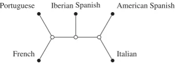
Fig. 1. Quintet treeT5relating five Romance languages.

Latent tree model selection techniques often presuppose that the data generating process is driven by some latent tree model, so the appropriateness of any such model is assessed only relative to other tree models. Knowing whether any latent tree model could adequately explain what is observed is pertinent in phylogenetic settings where, for example, the effect of a pos-sible horizontal gene transfer (Hao & Golding, 2008) makes any underlying such model dubi-ous.

By characterizing the covariance space related to Gaussian latent tree models, we can better assess the suitability of trees or the fit of a particular tree. In this paper we present the complete description of this model class by relating a particular model parameterization to the space of phylogenetic oranges (Engstr¨om et al., 2012;Gill et al., 2008;Kim, 2000; Moulton & Steel,

2004). Such a complete description had been known for a simple tree with only four leaves (Pearl & Xu,1987, Theorem 2) or for a star tree (Bekker & de Leeuw,1987). For a general tree, only the defining equations have been derived; seeSullivant(2008, Corollary 6·5).

Our method uses the description of Gaussian latent tree models in two scenarios. In the first we are interested in whether any latent tree model is a possible explanation for a given dataset. In the second we fix a latent tree model. In both scenarios the alternative hypothesis is the satu-rated model. We illustrate these methods in§5·3where we perform an exploratory search across language trees and in§5·4where we test whether a previously hypothesized phylogenetic tree fits data for certain yeast species. In both applications it is contentious whether the class of phy-logenetic trees is appropriate. This is addressed directly in our analyses without first fitting the model.

Let Z=(Zu)u∈U be a random vector whose components are indexed by the vertices of an undirected treeT =(U,E)with edge setE⊂U×U. The treeT induces a Gaussian tree model

N(T) for Z, which is a Gaussian graphical model onT (Lauritzen,1996,§5·2). For any two nodes u, v∈U, let ph(uv)denote the set of edges on the unique path betweenu andvin this tree. Then the modelN(T)is the collection of all multivariate normal distributions onR|U|for which Zu and Zv are conditionally independent given a subvector ZC whenever the setC⊂

U\{u, v}contains a node on ph(uv). For three nodesu, v, w∈U, the conditional independence ofZ_vandZ_w givenZuis equivalent toρvw=ρuvρuw. It follows that a normal distribution with correlation matrix R=(ρuv)belongs toN(T)if and only ifρuv=_e_∈_ph(_u_v)ρefor allu, v∈U, whereρe=ρuvwheneis the edge(u, v).

In this paper we study Gaussian latent tree models where we only observe the random vari-ables associated with the tree’s leaves. We henceforth denote the set of leaves of this tree byV

and associated leaf distributions asV-marginal distributions. A typical such evolutionary tree, of Romance languages, is displayed in Fig.1, where the observable, extant languages are repre-sented as its leaves.

DEFINITION1. The Gaussian latent tree model M(T)for the subvector X=(Z_v)_v_∈V is the

set of all V -marginal distributions of the distributions in N(T).

(4)

The parameterization ofM(T)is induced from the parameterization ofN(T)and is

ρi j=

e∈ph(i j)

ρe, i, j∈V. (1)

As the variancesσuu foru∈U\V never appear in this parameterization, without loss of gener-ality, we can assume they are equal to 1.

2. SEMIALGEBRAIC DESCRIPTION OF THE LATENT TREE MODEL

2·1. Tree metrics and phylogenetic oranges

LetT =(U,E)be a tree with leaf setV ⊆U. Associate to each edge a nonnegative number

de, which we interpret as the length of this edge. Then we can compute the distance between any two leavesi, j∈V asdi j=

e∈ph(i j)de. It is easy to check that a collection of such distances for all pairsu, v∈V forms a metric. The set of all metrics that arise in this way for allT with leaves labelled byV is called the space of tree metrics. We recall the following result.

THEOREM1 (Buneman,1974). A collection of positive numbers di j for i, j∈V forms a tree

metric if and only if for all, not necessarily distinct, i,j,k,l∈V we havemax(di k+djl,dil+

dj k)di j+dkl. Equivalently, for any three sums di k+djl, dil+dj k, di j +dkl, two are equal

and not less than the third. Moreover, if the tree metric inequalities hold, then genericallyT is uniquely identified.

In Theorem1the term generically means that the statement holds outside a set of measure zero corresponding to the vanishing of some edge lengthsde. A more precise statement is possible if we allow semi-labelled trees; seeSemple & Steel(2003,§7). A careful analysis shows that this generic tree is always binary, i.e., all its inner nodes have degree three. The triangle inequality follows from settingi, j,kdistinct andk=lin Theorem1, which in turn implies that every tree metric is a metric onV.

COROLLARY1. The space of tree metrics on a fixed treeT is the set of all metrics on V such

that for any four distinct leaves i, j,k,l such thatph(i, j)∩ph(k,l)= ∅, di k +djl=dil +dj k

di j+dkl.

Recall that ph(i, j)is the set of edges and hence, for example, for a star tree any four leaves

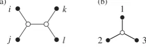
i,j,k,l satisfy ph(i, j)∩ph(k,l)= ∅. The condition ph(i, j)∩ph(k,l)= ∅ implies that the induced subtree overi, j,k,l, that is, the smallest connected subgraph ofT containingi, j,k,l, is a quartet tree as in Fig.2(a). This also explains the conditions of Corollary1.

Another closely related space defined over a tree is the space of phylogenetic oranges (Kim,

2000;Moulton & Steel,2004). For a fixed treeT this is the same parameterization (1) as the Gaussian latent tree model but where the edge correlationsρe are non-negative. The set of all points inRm(m−1)/2that arise in this way is denoted PO(T)and it forms a toric cube as defined inEngstr¨om et al.(2012). The union of all PO(T)is denoted by PO(V).

Let PO₊(T) and PO₊(V) respectively denote the subsets of PO(T) and PO(V) for which all coordinates are strictly positive; thus the corresponding edge correlationsρemust be strictly positive. The space of tree metrics on a fixed treeT is isomorphic to PO₊(T), with the isomor-phism given bydi j= −logρi j.

(5)

i

j

k

l 2

1

(a) (b)

3

Fig. 2. (a) A quartet treei j|kl. (b) Tripod tree.

THEOREM2. Let R=(ρi j)i,j∈V and suppose thatρi j0for all i, j∈V . Then:

(a) R∈PO(V)if and only if for every four not necessarily distinct elements i, j,k,l in V , at least two out of three productsρi kρjl,ρilρj k,ρi jρklare equal and less than or equal to the third.

Moreover, if this holds thenT with the property R∈PO(T)is generically identified uniquely; (b) for a fixed T, the space PO(T) has dimension |E|. This is described by the following set of constraints. For any four distinct elements i, j,k,l of V such thatph(i, j)∩ph(k,l)= ∅,

ρi kρjl=ρilρj kρi jρkl.Moreover, for any three distinct leaves i, j,k, the triangle inequality ρi jρi kρj k holds.

2·2. Latent tree models and phylogenetic oranges

We are now ready to derive the semialgebraic description of the model M(T). LetS₊(V)

denote the space of all symmetric positive definite|V| × |V|-matrices.

THEOREM3. Let T be a tree and let R=[ρi j]∈S+(V) be a correlation matrix. Then

R∈M(T)if and only if R=[|ρi j|]∈PO(T)andρi jρi kρj k0for any three distinct i, j,k∈V .

The proof is given in the Appendix.

Example1. LetT be the tripod tree in Fig.2(b). The space of correlation matrices inM(T)

is described by the inequalities

ρ12ρ13ρ230, |ρ12ρ13||ρ23|, |ρ12ρ23||ρ13|, |ρ13ρ23||ρ12|.

If ρ12, ρ13, ρ230 then by Theorem 2(b) the space described by the above inequalities

cor-responds to PO(T). There are three other sign patterns for ρ12, ρ13, ρ23 that ensure that

ρ12ρ13ρ230. For every such pattern we obtain a copy of PO(T). Quite remarkably, the space

of the correlation matrices in M(T)looks exactly like the three-dimensional slice of the corre-sponding binary latent class model; see Allman et al.(2015, Fig. 1). Such constraints cannot, in general, be neglected. For example, simple calculations show that the ratio of the volume of

M(T)to the volume of all 3×3 correlation matrices is only 2/π2≈0·2.

Based on Theorem2(b) and Theorem3we formulate the following result.

PROPOSITION1. IfT is a fixed tree then the space M(T)has dimension|V| + |E|. Let

be a covariance matrix with no zeros. Then ∈M(T) if and only if for any three distinct leaves i,j,k,

(σkkσi j−σi kσj k)(σj jσi k−σi jσj k)(σiiσj k −σi jσi k)0, (2)

and for any four distinct elements i, j,k,l of V such thatph(i, j)∩ph(k,l)= ∅,

σi kσjl σi jσkl =

σilσj k σi jσkl

1. (3)

[image:5.544.196.339.63.109.2]

(6)

This full algebraic and semialgebraic description can be viewed as a generalization of the main results inBekker & de Leeuw(1987) andPearl & Xu(1987) from star trees to general trees. An analogous description of the second order moments for binary latent tree models was given in

Zwiernik & Smith(2011). The similarity of both descriptions arises because the parameterization of correlations in the binary latent tree model is precisely (1); see Zwiernik & Smith (2011, Lemma 4·1).

3. USING SEMIALGEBRAIC CONSTRAINTS

We now describe how the semialgebraic constraints can be used to give an indication of tree-compatibility. Here the constraints in (2), which hold for every tree topology, will be called tree-compatibility constraints. A test based on these constraints can be used as an effective preliminary assessment tool to inform whether it is legitimate to proceed to a more complex tetrad analysis as described in §5. For a fixed T we can further extend our test by including the inequality constraints in (3). The resulting constraints are calledT-compatibility constraints. A test of fit based on such constraints is called a tree-compatibility orT-compatibility test as appropriate.

A straightforward but effective assessment of T-compatibility constraints can be obtained from the posterior probabilities by applying an inverse Wishart prior on the sample covariance. Ifˆ is a sample covariance matrix based on a sampleX of sizenfromNm(0,C), then the esti-mated scatter matrix is calculated as S=nˆ =X XT_{, where} _XT_{is the transpose of}_X_{, which is} Wishart distributed,S∼Wm(n,C)(Wishart,1928). A common prior distribution for unknown covarianceCis inverse Wishart,W_m−1(n0,C0), e.g.,Gelman et al.(2013),Carlin & Louis(2008)

andRoverato(2002). The inverse Wishart prior is conjugate, so the posterior density p(C|X)is inverse WishartW_m−1(n0+n,C0+S). As inRoverato(2002), forC0the identity matrixI|V|can be used and lettingn0=mensures that the inverse Wishart prior density has a valid number of

degrees of freedom. Then covariance matrices can be sampled from the conditional distribution ofC given X and each draw standardized to form a correlation matrix and then tested against the constraints. After N such draws from the posterior distribution, an estimate of the posterior probability thatC satisfies the positivity constraint can be obtained. Of course other choices of families of priors could be chosen instead, for example the scaled inverse Wishart distribution (O’Malley & Zaslavsky,2008), or we could use a strategy that models correlation and covari-ance separately (Barnard et al.,2000). However, these alternatives bring additional computational cost and complexity. An entirely different approach focusing on Bayesian methods could involve adapting the work on inequality-constrained hypotheses to assess tree-compatibility, seeVan de Schoot et al.(2012),Gu et al.(2014) andGardner et al.(2014).

In Example1, an estimate of the probability ofC satisfying the semialgebraic structure of

M(T)can be constructed using indicator functions. For each drawl from the relevant inverse Wishart posterior distribution forˆ, the following identity is evaluated:

r₁₂₃l ()ˆ =1{(σ˜33σ˜12− ˜σ13σ˜23)(σ˜22σ˜13− ˜σ12σ˜23)(σ˜11σ˜23− ˜σ12σ˜13)0}

whereσ˜i j (i, j=1,2,3)are the covariances corresponding to covariance drawlof the posterior, the indexlbeing dropped for simplicity. The posterior probability of tree-compatibility is thus estimated using

R123()ˆ =

1

N

l=1

r₁₂₃l ().ˆ (4)

(7)

For a tree with four variables such that ph(1,2)and ph(3,4)do not intersect, the remaining test associated with the inequality constraints is

R12|34()ˆ =

1

N

l=1

1{ ˜σ14σ˜23− ˜σ12σ˜340}1{ ˜σ13σ˜24− ˜σ12σ˜340}

1i<j

<k4

r_{i j k}l ().ˆ

These sampling approaches do not extend to the algebraic constraints because the set of draws from the posterior satisfying an equality constraint will have zero probability. Thus an alternative approach is needed that uses sample distributions of the minors of a covariance matrix.

4. THE SAMPLE DISTRIBUTION OF ALGEBRAIC CONSTRAINTS

From§3and Theorem2(b), the signs of tetrad constraintsσi kσjl −σilσj kand other quadratic binomials of the formσiiσj k−σi jσi k provide essential information about whether a Gaussian distribution lies inM(T). These types of constraints can be realized as minors of the covariance submatrix, that is det(i j,kl)and det(i j,i k)wherei j,kl denotes the 2×2 submatrix of with rowsi and j and columns k andl. Let M2 denote the set of all subsets of{1, . . . ,m}of

cardinality two. We now propose the following estimator of the value of det(CI,J)forI,J ∈M2,

QI,J =

1

n(n−1)det(SI,J). (5)

We note fromDrton et al.(2008, Corollary 4·2) that QI,Jis an unbiased estimator of det(CI,J). In what follows we provide the covariances between different QI,J. For anm×m matrix

A, let A(2)denote the matrix with rows and columns indexed by elementsM2 whose(I,J)th

element is the corresponding minor det(AI,J). With this notation, the matrix whose elements are the estimatorsQI,J isS(2)/n(n−1).

There is no simple explicit formula for covariances of various 2-minors, but they can be com-puted if the true distributionC is known. FromDrton et al.(2008, Proposition 3·3),

cov(S(2))=(C1/2)(2)⊗(C1/2)(2)cov(W(2))(C1/2)(2)⊗(C1/2)(2), (6)

whereWhas the standard Wishart distributionWm(n,I)and⊗is the Kronecker product. In the rest of this section we provide a complete description of the covariance matrix cov(W(2)). Our discussion followsDrton et al.(2008, Example 4·6). This gives the same deriva-tion for the casem=4. We show below that the generalization tom4 is straightforward.

The matrix cov(W(2)) has many symmetries that we want to exploit. For all I,J ∈M2,

detWI,J=detWJ,I, so

cov{det(WI,J),det(WK,L)} =cov{det(WJ,I),det(WK,L)} =cov{det(WK,L),det(WI,J)}.

We can therefore, without loss of generality, consider only unordered pairs of sets(I,J), where

I = {i, j}andJ = {k,l}withi< j,k<land eitheri<kori=kand jl.

Let AB=(A\B)∪(B\A)be the symmetric difference of two sets. We split the rows and the columns of cov(W(2))into blocks according to the values ofIJ andKL. With this con-vention, byDrton et al.(2008, Corollary 4.2 and Proposition 3.4), cov(W(2))is a block-diagonal matrix. Therefore, it is enough to describe its diagonal blocks. Since|IJ| ∈ {0,2,4}, we have

(8)

three types of blocks. We first describe the block corresponding toIJ=KL= ∅, or equiv-alently I =J,K=L. This block forms am(m−1)/2×m(m−1)/2-matrix that satisfies:

cov{det(WI,I),det(WK,K)} = ⎧ ⎪ ⎨ ⎪ ⎩

0, |I ∩K| =0,

2n(n−1)2, |I ∩K| =1, 2n(2n+1)(n−1), I =K.

We now have m(m−1)/2 blocks corresponding to IJ =KL= {i, j} for 1i< jm. Every such block is an (m−2)×(m−2) matrix, where I = {i,k}, J= {j,k}, K= {i,l},

L= {j,l}for somekl∈ {1, . . . ,m}\{i, j}. All of these matrices have two types of elements. The diagonal entries, k=l, equaln(n+2)(n−1). The off-diagonal elements, k<l, up to a sign, aren(n−1)2. The sign depends on the relative order ofi, j,k,l. By Drton et al.(2008, Theorem 4.5), the sign is positive ifk<i< j<l. Now a simple sign analysis shows that the sign is negative only if eitheri<k< j<lork<i<l< j. This yields

cov{det(Wi k,j k),det(Wil,jl)} = ⎧ ⎪ ⎨ ⎪ ⎩

n(n+2)(n−1), k=l,

−n(n−1)2, i<k< j<lork<i<l< j, n(n−1)2, otherwise.

Finally, there are m(m−1)(m−2)(m−3)/24 blocks corresponding to IJ= {i, j,k,l}, where 1i< j<k<lm. Each such block is a 3×3 matrix of the form

i j,kl i k, jl il, j k

_a _b ₋_b

· a b

· · a

wherea=2n(n−1)andb=n(n−1).

5. QUARTETS AND APPLICATIONS OF TETRAD ANALYSES

5·1. The method of quartets

For any four distinct leavesi, j,k,l∈V we say thatqi j,kl=i j|klforms a quartet ofT if the paths ph(i, j)and ph(k,l)are disjoint, cf. Fig.2(a). A binary treeT displays the set of quartetsQ if each quartetq∈Qis a quartet ofT. A set of quartetsQis said to determineT ifT displaysQ andT is the unique tree displayed byQ(Semple & Steel,2003); the set of all quartets displayed by T is denoted byQ_T. Quartets can be considered to be fundamental components of binary trees; seeDress et al.(2012) for more details. A setQ_T is said to be minimal if there exists no elementq∈Q_T such thatQ_T\{q}determinesT.Gr¨unewald et al.(2008, Theorem 2.4) provides the minimum size of anyQ_T, i.e., the size of the smallest minimal defining quartet set, which for a binary tree is just the number of internal edges ofT. Furthermore,Semple & Steel(2003, Theorem 6.8.8) provide a quick method for constructing minimal defining sets of quartets that define binary phylogenetic trees.

Let V ⊂U be such that V = {i, j,k,l}, where these elements are distinct. Consider three random variables Qi k,jl, Qil,j k and Qi j,kl as defined in (5). By Theorem 2, if a tree model holds, then the mean of one of the three will be zero and the other two means will be equal up to sign. So these QI,J can be used to test the algebraic constraints in Proposition1.

(9)

Here we focus on testing the vanishing tetrads, i.e., testing whether the quartetqi j,kl is dis-played inT given the data. To test a particular binary treeT, a setQ_T is required, i.e., a set of quartetsQthat determinesT. The number of edges ofT is 2m−3 and so the Gaussian latent tree model onT has codimensionm(m−1)/2−(2m−3). This means that to test a model, we need to work with quartet systemsQ_T of size quadratic inm. On the other hand if we believe that the data come from a latent tree model, then to only find the corresponding treeT we can work with any minimal quartet system determiningT, and these are of sizem−3, the number of internal edges. This makes a big difference for larger trees.

In practice, one may wish to selectQ_T such that it is minimal of sizem(m−1)/2−(2m−3),

i.e., it contains no redundant quartets, because otherwise the covariance of minors matrix may be close to being singular; seeBollen & Ting(1993). However, there may be no obvious reason to select one minimal defining quartet setQ_T over another. In such cases one approach is to randomly select a number of sets to assess the robustness of the results; seeBollen & Ting(1993). For eachqi j,kl∈QT consider the correspondingQi j,kl as in (5) and define QT =[Qi j,kl] to be the vector of these Qi j,kl. We write Qˆi j,kl for the sample means of the observations of Qˆi j,kl. Since Qˆ_T is a consistent estimator of Q_T (Drton et al.,2007), as the sample size n tends to infinity any treeT is uniquely identified by thei, j,k,lsuch thatE(Qˆi j,kl)=0.

To standardize the data we use the sample covariance matrix ˆQ_T which has dimension

p= |Q_T|, or we can use its proxy˜Q_T, obtained by recycling cov(W(2))computed in§4and replacingC in (6) with the sample covariance of original variablesˆ. The matrix˜Q_T can be obtained much more efficiently thanˆQ_T. An appropriate simultaneous test statistic (7) is pro-vided inBollen & Ting(1993),

T = ˆQT

T ˆ−Q1_T QˆT. (7)

AsT is constructed with palgebraically independent quartets, its asymptotic distribution is χ2

p. Compare (7) withBollen & Ting(1993, (20)) where theirtt is the covariance ofn1/2Qˆ_T. Here the sample sizen is incorporated implicitly throughˆ−_Q1

T so (7) provides a significance

test for the equality constraints in (3), where the required moments ofQI,J are given in§4. This provides a quick method for assessing whether a Gaussian dataset appears consistent with the algebraic constraints associated with any tree model.

In deriving the asymptotic distribution of (7) we implicitly assume that the true covariance matrix is a sufficiently regular point of the given tree model. In practice, it is enough to assume that the true covariance matrix contains no zeros; seeDrton et al.(2016a) andDrton et al.(2016b,

§5).

Hypothesis testing for vanishing tetrads can be used for both confirmatory tetrad analysis and for exploratory tetrad analysis. There are many algorithms for obtaining candidate trees, for instance seeJunker & Schreiber(2011) andSung(2009) for surveys of methods. However, often there is no way to assess the suitability of the final tree. Confirmatory tetrad analysis takes a candidate tree and provides an absolute rather than relative value as to how well the data support the purported tree.

In the case of a large tree it is infeasible to test all quartets at once, but it is straightforward and very stable to test single quartets or a small subset of them. One advantage of this approach is that it allows us to identify easily certain macrostructures of the tree which may lead to more robust techniques for finding the underlying tree. We now illustrate confirmatory and exploratory techniques for simulated data and some linguistics datasets.

(10)

Value of the statistic

Density

0 1 2 3 4 5 6 7 0·0

1·0

2·0 (a) (b)

(c) (d)

Density

0·0 1·0 2·0

0 5 10 15 20

Density

0 2 4 6 8

0·0 0·2 0·4

Density

0 2 4 6 8 10 12 0·00

[image:10.544.99.457.58.294.2]

0·10 0·20 0·30

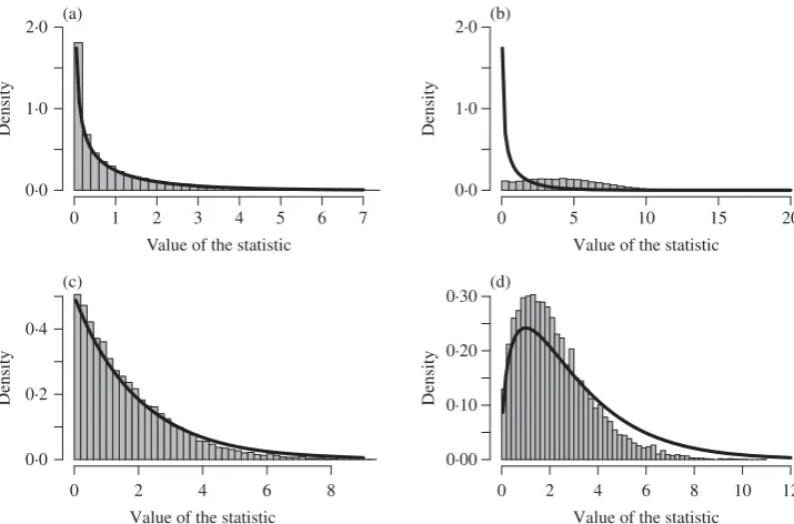
Fig. 3. Illustration of the simulations in§5·2. One hundred observations are generated from a random matrix in the tree model for the quintet tree 12|5|34 and the corresponding test statistic is computed. This procedure is repeated 10 000 times. In each panel we compare the sample distribution of a test statistic against its theoretical distribution. In (a) we test a single tetrad 12|34. In (b) we test a single false tetrad 13|24. In (c) we test two tetrads 12|35, 15|34, and in (d) we test a minimal set of quartets

defining the true quintet tree. The solid lines are densities ofχ₁2,χ₁2,χ₂2, andχ₃2respectively.

5·2. Basic simulations for the method of quartets

In this section we provide a basic analysis of the methods discussed in the previous section. The only difference from the previous applications of this method in other contexts is that in (7) we explicitly replaced the sample covariance of the tetrads with˜Q_T as explained in§5·1. The data in our simulations come from the quintet tree model 12|5|34; cf. Fig.1.

We first randomly choose the true covariance matrixCby sampling the edge correlations uni-formly from the interval [1/2,1]. Given this random true covariance matrix, we can now repeat the following evaluation procedure 10 000 times. We samplen=100 points from the given distri-butionC. In this scenario, standard packages that might be used to find the maximum likelihood estimate, such as the sem package (Fox et al.,2014;R Development Core Team,2016), are unsta-ble. On the other hand any set of quartets can be easily tested, without fitting the model. Moreover, the sample distribution of the test statistic is already very close to the asymptotic distribution, even when the sample size is only about twice the dimension of the model, though of course the power of the test will then be much lower.

In Fig.3we compare simulated values of test statistics of the form (7) with their asymptotic distributions. Figure 3(a) depicts the statistic built on a single tetrad constraint for the quartet 12|34. This constraint holds for the data-generating distribution and therefore the test statistic should have asymptoticχ₁2distribution. The histogram is very close to the theoretical distribu-tion. For comparison, Fig. 3(b) shows the sample distribution of the same test statistic for the quartet 13|24. This constraint does not hold for the data-generating distribution and the sample distribution of the corresponding test statistic is very far fromχ₁2. The test statistic can easily be set up for any subset of quartets. In Fig.3(c) we plot the test statistic to test two quartets 12|35

(11)

and 15|34. This is the minimal set of quartets that identifies the quintet tree 12|5|34. This means that these two particular quartets will not be simultaneously satisfied for any other tree model. Again, the sample distribution lies very close to the asymptoticχ₂2distribution.

In Fig. 3(d) we test simultaneously a minimal set of quartets 12|34, 12|35, 15|34 defining the quintet tree model. In this case the sample distribution of the test statistic also lies close to χ₃2 with a slightly smaller variance, because the true distribution is closer to a mixture of χ2_{-distributions; thus the test based on our statistic is typically more conservative. To obtain a}

bet-ter understanding of its performance we compare it with the structural expectation-maximization algorithm (Friedman et al.,2002) as applied to Gaussian latent tree models. This algorithm tries to find the tree that gives the maximum value of the likelihood function. However, like the stan-dard expectation-maximization algorithm, it often gets stuck in a local maximum. In our sim-ulations we generated 100 datasets from the given quintet model. If the sample size n=60, then for our particular choice of a correlation matrix with all edge correlations equal to 0·7, we obtained the correct tree only 68 out of 100 times. On the other hand, our tetrad method always confirms the correct tree for any significance level smaller than 0·1. Ifn=200 then the struc-tural expectation-maximization algorithm was correct 99 out of 100 times, and again our quar-tet method was always correct. We emphasize that in a less ideal situation, for example, when some edge correlations are small, or in the presence of partial misspecification, the structural expectation-maximization algorithm will perform poorly because the likelihood function is less stable. In contrast, our computations show that the quartet method tends to be much more robust.

5·3. Exploratory tetrad analysis example: linguistics

Consider now the linguistic dataset from Shiers et al. (arXiv:1410.0813), which comprises phonetic functional spectrogram data from French, Italian, Portuguese, and two forms of Span-ish, namely American and Iberian. Acoustic data have provided new insights into language devel-opment (Bouchard-Cˆot´e et al.,2013;Aston et al.,2010). Here the evolutionary dependencies between spoken numbers are studied, with each extant language treated as a leaf vertex. The high dimensional spectrogram data are projected from 8100 dimensions to 15 dimensions using a variant of canonical variate analysis, see Shiers et al. (arXiv:1410.0813). Each of the 15 canon-ical components projects the mean word data to obtain 15 new datasets referred to as canoncanon-ical scores. Each canonical component accounts for a particular combination of phonetic variation and each set of canonical scores is considered independently. This gives us the flexibility to hypothesize different evolutionary relationships for different aspects of the speech. For each set of canonical scores a 5×5 covariance matrix is calculated between the five languages. Royston’s multivariate normality test (Royston,1983) does not reject Gaussianity at the 0·01 level for any of these 15 sets of scores.

We sampled 105covariance matrices from the inverse Wishart posterior for each of the sample covariancesˆ1, . . . ,ˆ15. We then performed a tree-compatibility test with respect to the

positiv-ity constraint implied by the triangle inequalities in Theorem2(b) for each canonical component. We identify four such components, the first, fourth, sixth, and second, with high posterior prob-abilities, respectively 1, 0·89, 0·77 and 0·74, which warrant further investigation.

For the quintet tree in Fig. 1, there are 15 different labelled binary trees to test. In order to test a particular configuration of labels we construct a set of minimal defining quartetsQfor the quintet tree as referenced in§5·1; in the case of the quintet tree this smallest minimal set is two. For each of the four dimensions of interest, using the sampling distributions given in§4and the test statistic (7) with two degrees of freedom, a p-value can be calculated for each of the 15 non-isomorphic trees with languages as leaves. To retain an overall significance rate of less

(12)

S. kudriavzevii K. waltii

S. bayanus

S. mikitae

[image:12.544.193.363.60.128.2]

S. cerevisiae

Fig. 4. Quintet treeT5of yeast species (Marcet-Houben & Gabald´on,2009).

than 0·05 a Bonferroni correction (Dunn,1961) is applied such that the significance level is set at 0·05/15≈0·0033 per test. If more than one tree is not rejected then the candidate tree pro-posed by exploratory tetrad analysis is that with the highest p-value. We find that multiple trees exceed the threshold for all four components. The highest p-values for the first, second, fourth and sixth components were 0·524, 0·960, 0·775 and 0·902 respectively relating to the candidate trees: 12|4|35, 13|5|24, 14|2|35, and 23|1|45 respectively with coding 1=French, 2=Italian, 3=Portuguese, 4=American Spanish, 5=Iberian Spanish.

For illustration we focus on the candidate tree for the second component, which is displayed in Fig1. It is known from the analysis and expert interpretation in Shiers et al. (arXiv:1410.0813) that this component is likely to relate to variation in vowel sounds, nasality, and the lip rounding of language speakers. By isolating these phonetic features and identifying a tree that fits the data we can gain insights which may have otherwise been obscured. For example, from this particu-lar analysis we could hypothesize that the differences in nasality of Italian and French evolved independently conditional on the common ancestor of Spanish and Portuguese. In combination with expert judgement, such statements can provide good starting points for further analyses of these features in relation to a specified tree.

5·4. Confirmatory tetrad analysis example: biology

We next consider growth curves for five yeast species each observed in the same 96 envi-ronments, each species with at least two replicates. The growth was recorded at approximately six-minute intervals over a period of just over 26 hours. These species have been studied before (Marcet-Houben & Gabald´on,2009) and a phylogeny has been suggested as in Fig.4. However,

Libkind et al.(2011) hypothesize thatS. bayanusis a hybrid involvingS. cerevisiae. This alter-native hypothesis would violate the tree assumption. Previous research has indicated that for the studied yeast species there is positive correlation between growth-related phenotypic variation and genotypic phylogenetic relationships, e.g.,Liti et al.(2009) andWarringer et al.(2011). This leads us to consider the yeast growth-curve data to investigate evolutionary questions. We carried out a confirmatory tetrad analysis to assess whether the proposed tree structure inMarcet-Houben & Gabald´on(2009) was reflected in any aspects of the growth data.

To pre-process the data, a smoothed cubic spline basis was fitted to each growth vector, result-ing in a set of functional data objects which were then regularly evaluated to obtain comparable discretized representations. Mean vectors were then calculated for each species and environment and then these were standardized to remove mean environmental effects. We then performed a principal component analysis across species to identify the core variability of the growth curves. The first four components account for over 99% of variability. More detailed analysis, not reported here, can help interpret these components. For example, the first component relates only to growth variation in hours 10 to 26, whereas the second component relates to growth variation peaking at 12 hours with opposite growth variation from 18 hours onwards.

(13)

For each of the mean species projections in these dimensions, the sample covariance matrix was constructed. As a first step, the inverse Wishart approach specified in (4) was implemented. Recall that the tripod constraints are tree-compatibility constraints and thus require no tailoring to a specificT. Hence, these can be used very simply to narrow the list of components to test as part of a confirmatory tetrad analysis. The tree-compatibilities for the first four components were 31%, 2%, 18%, and 3% respectively. Thus, we consider the first and third components worth investigating further via confirmatory tetrad analysis forT-compatibility.

The results of the confirmatory tetrad analysis forT5-compatibility, see Fig.4, gave p-values

0·721 and 0·955 for the first and third components. To double-check these results we repeated the test using the bootstrapping strategy outlined inBollen & Stine(1992). The results were very sim-ilar, with p-values of 0·729 and 0·921 respectively. The confirmatory tetrad analysis and inverse Wishart simulation results both gave upper bounds onT5-compatibility, but on balance we

con-cluded that the first and third components wereT5-compatible. Therefore, the class of Gaussian

latent tree models does appear suitable for modelling some aspects of these yeast species’ growth curves. However, for features relating to components 2 and 4, there is some evidence to support the exploration of a wider model class that could accommodate the hybrid hypothesis described inLibkind et al.(2011).

6. DISCUSSION

Understanding the complete description of the correlation space associated with Gaussian latent tree models suggests a number of useful tools for assessing tree-compatibility either on a class basis or for a specified tree. Some of the methods described in this paper are particularly use-ful as part of an exploratory analysis for defining the relevant model search space, whereas others are ideal as a final check of the conclusions of a model search. The complete semialgebraic struc-ture of the correlation space has not been used elsewhere for assessing tree-compatibility of data, though the positivity constraint has been used previously; see Shiers et al. (arXiv:1410.0813). Incorporating a prior such as the inverse Wishart and sampling from the posterior distribution allows probabilistic conclusions about the model. This provides a more nuanced answer than a simple assessment of inequalities via the plugging in of covariance point estimates, and enables two or more incompatible but plausible trees to be compared.

Although our results are focused on Gaussian models, they can be extended to more gen-eral scenarios. Gaussian tree models can be thought of as linear structural equation models with Gaussian errors. If the errors are instead non-Gaussian but with finite variance, the covariance matrices will still obey the same constraints as in the Gaussian models. This means that our pro-cedure can be used for basic model assessment also for non-Gaussian data given the second order moments exist.

One important practical consideration is the scalability of these methods. Techniques employing the semialgebraic constraints can be adapted to a larger number of variables reason-ably well. For a confirmatory tetrad analysis the biggest computational cost is the calculation of the covariance of minors, which for pobserved random variables has dimension of order p4, and can become prohibitive. For example, if 8GB of RAM is allocated for a single matrix, the limit of pis approximately 25 even if redundant rows and columns are removed from the matrix. However, much larger pcan be considered by calculating the relevant statistics for each quartet marginally. Then the covariance matrix of minors has dimension only 36 and the memory can be released once each quartet has been tested. In either case, the final memory requirement could further be reduced with programming that takes advantage of symmetries and sparseness. In a similar vein, to extend the scope of exploratory tetrad analysis to a greater number of variables,

(14)

one strategy is to only assess single quartets in the first instance and use these results to reduce the set of possible trees. Given the effectiveness of the quartet testing with even small sample sizes, this approach seems sensible and to have significant advantages over methods that require a whole model to be tested at once.

ACKNOWLEDGEMENT

We are grateful to both referees for comments that substantially improved the presentation of the paper. Nathaniel Shiers acknowledges the support of the Economic and Social Research Council. Piotr Zwiernik was supported by the European Union 7th Framework Programme. John Aston was supported by the Engineering and Physical Sciences Research Council. The authors wish to thank Pantelis Hadjipantelis for pre-processing the linguistic data, John S. Coleman for interpretation of the linguistic analysis, and Chris Knight for provision of the yeast data.

APPENDIX

Proofs

Proof of Theorem2. Assume first that all correlationsρi j are strictly positive, that is R∈PO+(V)or

R∈PO₊(T). We use the fact that PO₊(V)is isomorphic to the space of tree metrics, whose constraints are given in Theorem1and Corollary1. Translating these constraints viadi j= −logρi j gives exactly the

constraints in the proposed theorem. These constraints describe a closed set, which is the smallest closed set containing PO₊(V), so it is enough to show that the closure of PO₊(T)is equal to PO(T). This follows from the fact that PO(T)is a toric cube and, byEngstr¨om et al.(2012, Theorem 1), every toric cube is equal to the closure of its interior.

Proof of Theorem3. IfR∈M(T)then eachρi j has representation (1). Thus|ρi j| =

e_∈ph₍i j₎|ρe|and

henceRalso lies in PO(T). To show thatρi jρi kρj k0 consider the induced subtree overi,j,k, that is,

the smallest connected subgraph of T containing verticesi,j,k. This subtree necessarily has a unique vertexvthat lies on the intersection of paths ph(i j), ph(i k)and ph(j k). Moreover, by (1),

ρi jρi kρj k=

e∈ph(i j)

ρe

e∈ph(i k)

ρe

e∈ph(j k)

ρe=

e∈ph(iv)

ρ2

e

e∈ph(jv)

ρ2

e

e∈ph(kv)

ρ2

e0.

To prove the reverse implication, we note that every correlation matrix in PO(T)has, after permuting rows and columns, a block diagonal structure with strictly positive elements in each block. Consider first the case when all elements ofRare nonzero, that is,Rhas strictly positive entries. Distinguish one node inVand label it as 1. LetDbe a diagonal matrix such thatDii= −1 ifρ1i<0 andDii=1 ifρ1i>0. IfR∈M(T)

then also D R D lies in M(T)because M(T)is invariant with respect to all diagonal transformations. Moreover, it holds that R=D R Dbecause D11Diiρ1i= |ρ1i|for alli∈V\{1}andDiiDj jρi j= |ρi j|for

i,j∈V\{1}. This last equality follows from our assumption thatρ1iρ1jρi j0 so that the sign ofρ1iρ1j

is equal to the sign ofρi j. Now, sinceR∈PO(T)⊂M(T)andR=D RDwe also have thatR∈M(T).

The analysis of the case when Ris block diagonal will be omitted.

REFERENCES

ALLMAN, E. S.,RHODES, J. A.,STURMFELS, B. &ZWIERNIK, P. (2015). Tensors of nonnegative rank two.Lin. Algeb. Applic.473, 37–53.

ASTON, J. A. D.,CHIOU, J.-M. &EVANS, J. P. (2010). Linguistic pitch analysis using functional principal component mixed effect models.Appl. Statist.59, 297–317.

BARNARD, J.,MCCULLOCH, R. &MENG, X.-L. (2000). Modeling covariance matrices in terms of standard deviations and correlations, with application to shrinkage.Statist. Sinica10, 1281–312.

BEKKER, P. A. &DELEEUW, J. (1987). The rank of reduced dispersion matrices.Psychometrika52, 125–35.

(15)

BOLLEN, K. A. &STINE, R. A. (1992). Bootstrapping goodness-of-fit measures in structural equation models.Sociol. Meth. Res.21, 205–29.

BOLLEN, K. A. &TING, K. (1993). Confirmatory tetrad analysis. InSociological Methodology, P. Marsden, ed., vol. 23. Cambridge, USA: Blackwell Publishing, pp. 147–75.

BOUCHARD-CˆOT´E, A.,HALL, D.,GRIFFITHS, T. L. &KLEIN, D. (2013). Automated reconstruction of ancient languages using probabilistic models of sound change.Proc. Nat. Acad. Sci.110, 4224–9.

BUNEMAN, P. (1974). A note on the metric properties of trees.J. Combin. Theory Ser. B17, 48–50.

CARLIN, B. P. &LOUIS, T. A. (2008).Bayesian Methods for Data Analysis. Boca Raton, USA: Chapman & Hall/CRC, 3rd ed.

CHOI, M. J.,TAN, V. Y. F.,ANANDKUMAR, A. &WILLSKY, A. S. (2011). Learning latent tree graphical models.J. Mach. Learn. Res.12, 1771–812.

DRESS, A.,HUBER, K. T.,KOOLEN, J.,MOULTON, V. &SPILLNER, A. (2012).Basic Phylogenetic Combinatorics. Cambridge, UK: Cambridge University Press.

DRTON, M.,LIN, S.,WEIHS, L. &ZWIERNIK, P. (2016a). Marginal likelihood and model selection for Gaussian latent tree and forest models.BernoulliTo appear.

DRTON, M.,MASSAM, H. &OLKIN, I. (2008). Moments of minors of Wishart matrices.Ann. Statist.36, 2261–83. DRTON, M.,STURMFELS, B. &SULLIVANT, S. (2007). Algebraic factor analysis: tetrads, pentads and beyond.Prob.

Theory Rel. Fields138, 463–93.

DRTON, M.,XIAO, H.ET AL. (2016b). Wald tests of singular hypotheses.Bernoulli22, 38–59. DUNN, O. J. (1961). Multiple comparisons among means.J. Am. Statist. Assoc.56, 52–64.

EISENSTEIN, J.,O’CONNOR, B.,SMITH, N. A. &XING, E. P. (2010). A latent variable model for geographic lexical variation. InProc.2010Conference on Empirical Methods in Natural Language Processing. Cambridge, USA. ENGSTROM¨ , A.,HERSH, P. &STURMFELS, B. (2012). Toric cubes.Rend. Circ. Mat. Palermo (2)62, 1–12.

FOX, J.,NIE, Z. &BYRNES, J. (2014).sem: Structural Equation Models. R package version 3·1-5.

FRIEDMAN, N.,NINIO, M.,PE’ER, I. &PUPKO, T. (2002). A structural EM algorithm for phylogenetic inference. J. Comp. Biol.9, 331–53.

GARDNER, J. R.,KUSNER, M. J.,XU, Z.,WEINBERGER, K. Q. &CUNNINGHAM, J. P. (2014). Bayesian optimization with inequality constraints. InPro. 31st Int. Conf. Machine Learning, E. P. Xing & T. Jebara, eds. Beijing, China. GELMAN, A.,CARLIN, J. B.,STERN, H. S.,DUNSON, D. B.,VEHTARI, A. &RUBIN, D. B. (2013).Bayesian Data Analysis.

Boca Raton, USA: Chapman & Hall/CRC, 3rd ed.

GILL, J.,LINUSSON, S.,MOULTON, V. &STEEL, M. (2008). A regular decomposition of the edge-product space of phylogenetic trees.Adv. Appl. Math.41, 158–76.

GRUNEWALD¨ , S.,HUMPHRIES, P. J. &SEMPLE, C. (2008). Quartet compatibility and the quartet graph.Electron. J. Combin.15, R103.

GU, X.,MULDER, J.,DEKOVIC´, M. &HOIJTINK, H. (2014). Bayesian evaluation of inequality constrained hypotheses. Psychol. Meth.19, 511–27.

HAO, W. &GOLDING, G. B. (2008). Uncovering rate variation of lateral gene transfer during bacterial genome evolu-tion.BMC Genom.9, 235.

JUNKER, B. &SCHREIBER, F. (2011).Analysis of Biological Networks. Hoboken, USA: Wiley.

KIM, J. (2000). Slicing hyperdimensional oranges: the geometry of phylogenetic estimation.Molec. Phylogenet. Evol. 17, 58–75.

KOLLER, D. &FRIEDMAN, N. (2009).Probabilistic Graphical Models: Principles and Techniques. Cambridge, USA: The MIT Press.

LAURITZEN, S. L. (1996).Graphical Models. Oxford, UK: Oxford University Press.

LAWRENCE, N. D. (2004). Gaussian process latent variable models for visualisation of high dimensional data.Adv. Neural Info. Proces. Syst.16, 329–36.

LIBKIND, D.,HITTINGER, C. T.,VALÉRIO, E.,GONÇALVES, C.,DOVER, J.,JOHNSTON, M.,GONÇALVES, P. &SAMPAIO, J. P. (2011). Microbe domestication and the identification of the wild genetic stock of lager-brewing yeast.Proc. Nat. Acad. Sci.108, 14539–44.

LITI, G.,CARTER, D. M.,MOSES, A. M.,WARRINGER, J.,PARTS, L.,JAMES, S. A.,DAVEY, R. P.,ROBERTS, I. N., BURT, A.,KOUFOPANOU, V.ET AL.(2009). Population genomics of domestic and wild yeasts.Nature458, 337–41. MARCET-HOUBEN, M. &GABALDON´ , T. (2009). The tree versus the forest: the fungal tree of life and the topological

diversity within the yeast phylome.PLOS ONE4, e4357.

MOULTON, V. &STEEL, M. (2004). Peeling phylogenetic ‘oranges’.Adv. Appl. Math.33, 710–27.

MOURAD, R.,SINOQUET, C.,ZHANG, N. L.,LIU, T. &LERAY, P. (2013). A survey on latent tree models and applications. J. Artif. Intel. Res.47, 157–203.

O’MALLEY, A. J. &ZASLAVSKY, A. M. (2008). Domain-level covariance analysis for multilevel survey data with structured nonresponse.J. Am. Statist. Assoc.103, 1405–18.

PEARL, J. &XU, L. (1987). Structuring causal tree models with continuous variables. InProc. 3rd Ann. Conf. Uncer-tainty Artif. Intel., J. Lemmer, T. Levitt & L. Kanal, eds. Corvallis, USA: AUAI Press.

R DEVELOPMENTCORETEAM(2016).R: A Language and Environment for Statistical Computing. Vienna, Austria: R Foundation for Statistical Computing. ISBN 3-900051-07-0,http://www.R-project.org.

(16)

ROVERATO, A. (2002). Hyper inverse Wishart distribution for non-decomposable graphs and its application to Bayesian inference for Gaussian graphical models.Scand. J. Statist.29, 391–411.

ROYSTON, J. P. (1983). Some techniques for assessing multivariate normality based on the Shapiro-WilkW.Appl. Statist.32, 121–33.

SEMPLE, C. &STEEL, M. (2003).Phylogenetics. Oxford, UK: Oxford University Press.

SULLIVANT, S. (2008). Algebraic geometry of Gaussian Bayesian networks.Adv. Appl. Math.40, 482–513.

SUNG, W.-K. (2009). Algorithms in Bioinformatics: A Practical Introduction. Boca Raton, USA: Chapman & Hall/CRC.

VAN DESCHOOT, R.,HOIJTINK, H.,HALLQUIST, M. N. &BOELEN, P. A. (2012). Bayesian evaluation of inequality-constrained hypotheses in SEM models using M plus.Struct. Equ. Model.19, 593–609.

WANG, Y.,ZHANG, N. L. &CHEN, T. (2008). Latent tree models and approximate inference in Bayesian networks. J. Artif. Intel. Res.32, 879–900.

WARRINGER, J.,ZORGO, E.,CUBILLOS, F. A.,ZIA, A.,GJUVSLAND, A.,SIMPSON, J. T.,FORSMARK, A.,DURBIN, R., OMHOLT, S. W.,LOUIS, E. J.ET AL. (2011). Trait variation in yeast is defined by population history.PLOS Genet. 7, e1002111–1.

WISHART, J. (1928). The generalised product moment distribution in samples from a normal multivariate population. Biometrika20A, 32–52.

ZWIERNIK, P. (2016).Semialgebraic Statistics and Latent Tree Models. Boca Raton, USA: Chapman & Hall/CRC. ZWIERNIK, P. &SMITH, J. Q. (2011). Implicit inequality constraints in a binary tree model.Electron. J. Statist.5,

1276–312.

[Received August2015. Revised June2016]