Eyewitness identification performance on lineups for distinctive suspects

(1)

warwick.ac.uk/lib-publications

A Thesis Submitted for the Degree of PhD at the University of Warwick

Permanent WRAP URL:

http://wrap.warwick.ac.uk/90153

Copyright and reuse:

This thesis is made available online and is protected by original copyright. Please scroll down to view the document itself.

Please refer to the repository record for this item for information to help you to cite it. Our policy information is available from the repository home page.

(2)

Eyewitness Identification Performance

on Lineups for Distinctive Suspects

by

Melissa Fay Colloff

A thesis submitted in partial fulfilment of the requirements for the

degree of

Doctor of Philosophy in Psychology

(3)

List of Tables

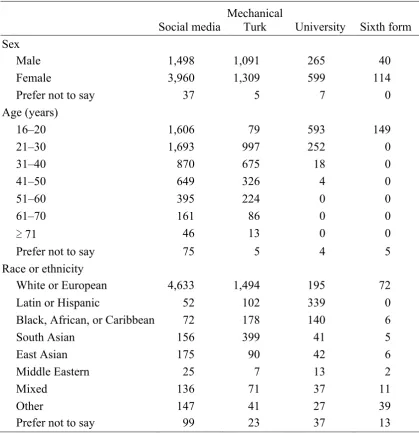
Table 1.1. Response Options in a Standard Eyewitness Identification Experiment .. 17! Table 2.1. Demographic Information For Social Media, Mechanical Turk,

University, and Sixth Form Samples ... 43! Table 2.2. Frequencies and Percentages of Identification Responses in the

Replication, Pixelation, Block, and Do-nothing Lineups ... 52! Table 3.1. Demographic Information For Young, Middle-aged, and Older Samples.

... 65! Table 3.2. Observed and Predicted Identification Responses in Each Confidence Bin

in the Fair Lineups for the Young, Middle-aged, and Older Adults ... 76! Table 3.3. Full and Constrained (d') Model Fits for the Young vs. Middle-aged,

Young vs. Older, and Middle-aged vs. Older Fair Lineup Comparisons ... 77! Table 3.4. Full, Reduced, and Constrained (Confidence Criteria) Model Fits for the

Young vs. Older Fair Lineup Comparisons ... 81! Table 4.1. Partial Area Under the Curve (pAUC) Statistics [and 95% Confidence

Intervals] ... 99! Table 4.2. Percentages (and Frequencies) of Descriptions in Each Coding Category.

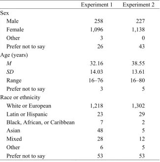
... 106! Table 5.1. Demographic Information for the Samples in Experiments 1 and 2 ... 124! Table 5.2. Mean (SE) Ratings of Distinctive Feature Similarity in Experiment 1 .. 128! Table 5.3. Percentages (and Frequencies) of Descriptions in Each Coding Category.

... 131! Table 5.4. Observed and Predicted Identification Responses in Each Confidence Bin

in the Low-variation, Moderate-variation, and Do-nothing Lineups in

Experiment 1 ... 142! Table 5.5. Full and Constrained (d') Model Fits for the Low-variation vs.

Moderate-variation, Low-variation vs. nothing, and Moderate-variation vs.

(8)

Table 5.7. Observed and Predicted Identification Responses in Each Confidence Bin in the Low-variation, High-variation, and Do-nothing Lineups in Experiment 2. ... 163! Table 5.8. Full and Constrained (d') Model Fits for the Low-variation vs.

High-variation, Low-variation vs. Do-nothing, and High-variation vs. Do-nothing Comparisons in Experiment 2 ... 164! Table A.1. Observed and Predicted Identification Responses in Each Confidence Bin in the Replication, Pixelation, Block, and Do-nothing Lineups ... 212! Table A.2. Full and Constrained (d') Model Fits for the Fair (Replication, Pixelation,

Block) vs. Unfair (Do-nothing) Lineup Comparisons ... 214! Table B.1. Frequencies of Identification Responses in Each Confidence Bin in the

Replication, Pixelation, Block, and Do-nothing Lineups ... 215! Table C.1. Partial Area Under the Curve (pAUC) Statistics [and 95% Confidence

Intervals] ... 218! Table C.2. Observed and Predicted Identification Responses in Each Confidence Bin

in the Replication, Pixelation, and Block Lineups for the Young, Middle-aged, and Older Adults ... 221! Table C.3. Full and Constrained (d') Model Fits for the Replication vs. Pixelation,

Replication vs. Block, and Pixelation vs. Block Comparisons in the Young, Middle-aged, and Older Adults ... 223! Table D.1. Observed and Predicted Identification Responses in Each Confidence Bin in the Unfair Lineups for the Young, Middle-aged, and Older Adults ... 226! Table D.2. Full and Constrained (d') Model Fits for the Young vs. Middle-Aged,

Young vs. Older, and Middle-aged vs. Older Unfair Lineup Comparisons .... 227! Table D.3. Full and Constrained (d') Model Fits for the Fair vs. Unfair Lineup

Comparisons in the Young, Middle-aged, and Older Adults ... 229! Table E.1. Frequencies of Identification Responses Made by the Young,

Middle-aged, and Older Adults in Each Confidence Bin in the Fair and Unfair Lineups. ... 230! Table F.1. Frequencies of Identification Responses Made by the Young-old and

(9)

Table G.1. Observed and Predicted Identification Responses in Each Confidence Bin in the Replication, Pixelation, Block, and Do-nothing lineups for the Non-distinctive and Distinctive Culprits ... 236! Table G.2. Full and Constrained (d') Model Fits for the Replication vs. Pixelation,

Replication vs. Block, Pixelation vs. Block, Replication vs. Do-nothing, Pixelation vs. Do-nothing, and Block vs. Do-nothing Comparisons for the Non-distinctive and Distinctive Culprits ... 237 Table G.3. Full and Constrained (d') Model fits for the Distinctive vs.

Non-distinctive Comparisons in the Replication, Pixelation, Block, and Do-nothing Lineups ... 239! Table H.1. Frequencies of Identification Responses Made in Each Confidence Bin in

the Replication, Pixelation, Block, and Do-nothing Lineups for the

Non-distinctive and Distinctive Culprits ... 240! Table I.1. Frequencies of Identification Responses in Each Confidence Bin in the

Low-Variation, Moderate-Variation, and Do-nothing Lineups in Experiment 1. ... 241! Table I.2. Frequencies of Identification Responses in Each Confidence Bin in the

(10)

List of Figures

Figure 1.1. (a) An unaltered image, (b) an example of how features (baldness, facial hair and blemishes) can be digitally added for replication lineups, and examples of how features can be concealed using (c) pixelation, or (d) block techniques. ... 21! Figure 1.2. Signal detection model with (a) a neutral, (b) a conservative, and (c) a

liberal decision criterion ... 26! Figure 1.3. Signal detection model for (a) a fair lineup and (b) an unfair lineup

(Wixted & Mickes, 2014) ... 29! Figure 1.4. Two hypothetical receiver operating characteristic (ROC) curves ... 31! Figure 2.1. Examples of (a) a replication lineup, (b) a pixelation lineup, (c) a block

lineup, and (d) a do-nothing (unfair) lineup ... 41! Figure 2.2. Receiver operating characteristic (ROC) curves for the fair (replication,

pixelation, block) and unfair (do-nothing) lineups ... 51! Figure 2.3. Confidence-accuracy curves for suspect identifications in the fair

(replication, pixelation, block) and unfair (do-nothing) lineups ... 54! Figure 3.1. Identification responses made by the young, middle-aged, and older

adults in fair and unfair (a) target-present and (b) target-absent lineups ... 71! Figure 3.2. Receiver operating characteristic (ROC) curves for the fair and unfair

lineups for the young, middle-aged, and older adults ... 72! Figure 3.3. Innocent and guilty distributions for (a) young, (b) middle-aged, and (c)

older adults using the best-fitting signal detection model parameters ... 78! Figure 3.4. The best-fitting signal detection model confidence criteria parameters (c1, c2, c3, c4, c5) for the young vs. older adults ... 80! Figure 3.5. Confidence-accuracy curves for suspect identifications in the fair and

unfair lineups ... 83! Figure 4.1. Receiver operating characteristic (ROC) curves for the replication,

(11)

Figure 4.2. Receiver operating characteristic (ROC) curves for the (a) replication, (b) pixelation, (c) block, and (d) do-nothing lineups in subjects who had watched a non-distinctive or a distinctive culprit ... 100! Figure 4.3. Identification responses made in replication, pixelation, block, and

do-nothing (a) target-present and (b) target-absent lineups, by subjects who had watched a non-distinctive or a distinctive culprit ... 104! Figure 4.4. Identification responses made in replication, pixelation, block, and

do-nothing (a) target-present and (b) target-absent lineups, by subjects who had watched a non-distinctive culprit, watched a distinctive culprit but failed to describe the feature, or watched a distinctive culprit and described the feature. ... 110! Figure 4.5. Confidence-accuracy curves for suspect identifications in the fair

(replication, pixelation, block) and unfair (do-nothing) lineups by subjects who had watched (a) a non-distinctive or (b) a distinctive culprit. ... 112! Figure 4.6. Confidence-accuracy curves for suspect identifications in the (a)

replication, (b) pixelation, (c) block, and (d) do-nothing lineups by subjects who had watched a non-distinctive or a distinctive culprit ... 114! Figure 5.1. (a) A sample culprit, (b) a low-variation lineup, (c) a moderate-variation

lineup, and (d) a do-nothing lineup in Experiment 1 ... 126! Figure 5.2. Receiver operating characteristic (ROC) curves for the low-variation,

moderate-variation, and do-nothing lineups ... 132! Figure 5.3. Receiver operating characteristic (ROC) curves for the low-variation,

moderate-variation, and do-nothing lineups in the (a) mugging and (b) graffiti videos ... 134! Figure 5.4. Identification responses made in low-variation, moderate-variation, and

do-nothing (a) target-present and (b) target-absent lineups ... 137! Figure 5.5. Foil, innocent suspect, and guilty suspect distributions for (a)

low-variation, (b) moderate-low-variation, and (c) do-nothing lineups using the best-fitting equal-variance signal detection model parameters ... 144! Figure 5.6. Confidence-accuracy curves for suspect identifications in the

low-variation, moderate-low-variation, and do-nothing lineups ... 146! Figure 5.7. (a) A sample culprit, (b) a low-variation lineup, (c) a high-variation

(12)

Figure 5.8. Receiver operating characteristic (ROC) curves for the low-variation, high-variation, and do-nothing lineups ... 154! Figure 5.9. Receiver operating characteristic (ROC) curves for the low-variation,

high-variation, and do-nothing lineups in the (a) mugging and (b) graffiti videos ... 156! Figure 5.10. Identification responses made in low-variation, high-variation, and

do-nothing (a) target-present and (b) target-absent lineups ... 160! Figure 5.11. Foil, innocent suspect, and guilty suspect distributions for (a)

low-variation, (b) high-low-variation, and (c) do-nothing lineups using the best-fitting equal-variance signal detection model parameters ... 165! Figure 5.12. Confidence-accuracy curves for suspect identifications in the

low-variation, high-low-variation, and do-nothing lineups ... 167! Figure C.1. Identification responses made by the young, middle-aged, and older

adults in replication, pixelation, block, and do-nothing (a) target-present and (b) target-absent lineups ... 217! Figure C.2. Receiver operating characteristic (ROC) curves for the replication,

pixelation, block, and do-nothing lineups for (a) young, (b) middle-aged, and (c) older adults ... 219! Figure F.1. Confidence-accuracy curves for suspect identifications made by

(13)

Acknowledgements

I am extremely grateful to all those people who have supported and

encouraged me throughout the course of my PhD. Primarily, I would like to thank Kimberley Wade, whose tireless guidance and support have been fundamental to both my research and future career. She is enthusiastic, honest, and always willing to go the extra mile to help her students. Kim is not only an outstanding supervisor, but is also an inspirational female scientist. I have learnt so much from her.

I also express my deepest gratitude to John Wixted for welcoming me into his lab and dedicating so much of his time to teach me signal detection statistics and modelling. My trip to San Diego was transformational and John’s wisdom and willingness to continue to educate me are invaluable.

Many thanks also to Elizabeth Maylor, Neil Stewart and Laura Mickes: Elizabeth for her unrivalled proof-reading, astute feedback, and ageing expertise; Neil Stewart for giving his valuable time to help me to programme my studies; and Laura for insightful discussions about ROC analysis. I am so grateful to Heather Flowe for believing that I was able to undertake a PhD and providing me with many rewarding and worthwhile opportunities along the way.

I must also acknowledge the Psychology Department at Warwick University for supporting me financially and allowing me to be surrounded by a group of

inspirational academics. Thank you also to all those people who made working in the office so enjoyable, and my lab mates—Sophie, Divya, and Harriet—for enduring countless practice presentations and draft papers. What a team!

(14)

Declaration

This thesis is submitted to the University of Warwick in support of my

application for the degree of Doctor of Philosophy. It has been composed by myself and has not been submitted in any previous application for any degree. The work presented (including data generated and data analysis) was carried out entirely by the author.

Inclusion of Published Work

Parts of this thesis have been published by the author.

Chapter 2 includes the following publication:

Colloff, M. F., Wade, K. A., & Strange, D. (2016). Unfair lineups make witnesses more likely to confuse innocent and guilty suspects. Psychological Science, 27, 1227–1239. doi:10.1177/0956797616655789

Dr Kimberley Wade contributed to the planning of this research and Dr Kimberley Wade and Dr Deryn Strange provided feedback on drafts of the manuscript.

Chapter 3 includes the following publication:

Colloff, M.F., Wade, K. A., Wixted, J.T., & Maylor, E. A. (in press). A signal-detection analysis of eyewitness identification across the adult lifespan. Psychology and Aging. doi:10.1037/pag0000168

Dr Kimberley Wade and Professor Elizabeth Maylor contributed to the planning of this research and Professor John Wixted assisted with the model fitting. All co-authors provided feedback on drafts of the manuscript.

In addition, Chapter 1, “Measuring discriminability”, paragraphs 2–4 and Figure 1.4, appear in Colloff et al. (2016). Chapter 1, “Gauging the likely accuracy of

(15)

Abstract

When constructing lineups for suspects with distinctive facial features (e.g., scars, tattoos, piercings), current police guidelines in several countries state that the distinctive suspect must not stand out. To this end, police officers sometimes artificially replicate a suspect’s distinctive feature across the other lineup members (replication); other times, they conceal the feature on the suspect and conceal a similar area on the other members by pixelating the area (pixelation), or covering the area with a solid rectangle (block). Although these three techniques are used

frequently, little research has examined their efficacy. This thesis investigates how the lineup techniques for distinctive suspects influence eyewitness identification performance and, in doing so, tests the predictions of a new model of eyewitness decision-making—the diagnostic-feature-detection model (Wixted & Mickes, 2014).

The research uses a standard eyewitness identification paradigm and signal detection statistics to examine how replication, pixelation, and block techniques influence identification performance: [1] compared to doing nothing to stop the distinctive suspect from standing out; [2] in young, middle-aged and older adults; and [3] when the culprit does not have the feature during the crime. It also examines [4] how variation in the way the suspect’s feature is replicated influences

identification performance.

(16)

Chapter 1 :

Introduction

Suppose that you were an eyewitness to a criminal event. Perhaps you saw a suspicious man in an area where you later learn a child has been abducted, or

perhaps you caught a glimpse of the young man when he grabbed the bag from your arm. Because you have seen the culprit, you are a valuable source of information for the police officers investigating the case (Kebbell & Milne, 1998). The investigating officers ask you to describe the culprit, and then, sometime later, perhaps days, but perhaps months, they ask you to attempt to identify the culprit from a lineup. In this lineup, the police officers place their suspect (who is either innocent or guilty) among other known-to-be-innocent lineup members, called foils. If you make a positive identification of the police suspect—you say: “That’s him!”—then this is likely to be interpreted as compelling evidence of guilt. Suspects who have been positively identified are more likely to be charged with the offence (Davis,

Valentine, Memon, & Roberts, 2015; Flowe, Mehta, & Ebbesen, 2011) and are more likely to be found guilty at court (Devlin, 1976; Pozzulo, Lemieux, Wells, &

McCuaig, 2006; Pozzulo, Lemieux, Wilson, Crescini, & Girardi, 2009) than those who have not. In short, eyewitness identification evidence plays a critical role in how a case proceeds through the Criminal Justice System.

The influence of eyewitness identification evidence in the Criminal Justice System is, however, concerning when we consider that memory can be unreliable. Eyewitness identification errors are frequent and can have profound consequences. In the United States since 1989, 344 convictions have been overturned on the basis of new DNA evidence. The Innocence Project estimates that over 70% of these wrongful convictions involved an eyewitness identification error—that is, the witness identified an innocent suspect (Innocence Project, 2016). Moreover, another type of identification error, failing to identify the culprit when he is in the lineup, can result in the real culprit being free to commit additional crimes. Subjects in

(17)

discussion). Although it is impossible to know the number of occasions in which a real culprit has been falsely acquitted because a witness failed to positively identify him, given these statistics, it appears that this type of error is also likely to be common.

Experimental research

As a result of the frequency of eyewitness identification errors, psychological scientists have conducted experimental studies in the lab to examine the factors that may enhance or impair eyewitness identification accuracy (Wright, 2006). In these studies, researchers usually employ a mock crime methodology. Subjects watch a staged crime—sometimes live, but usually one that has been videotaped—then, after a delay, are presented with a lineup and have to attempt to identify the culprit. In real life criminal investigations the ground-truth is unknown, because police officers can never be certain if their suspect is innocent or guilty. But in lab studies, this factor can be controlled and experimentally manipulated. Some subjects are presented with a lineup in which the real culprit is present (a target-present lineup), and the

remaining subjects are presented with a lineup in which the real culprit is absent (a target-absent lineup). Target-present lineups represent the real world situation in which the police suspect is guilty, whereas target-absent lineups represent the situation in which the police suspect is innocent. In both present and target-absent lineups, subjects can make one of three possible identification responses: they can identify the suspect, they can identify a foil, or they can reject the lineup and state that the real culprit is not present (see Table 1.1). In a target-present lineup, identifying the guilty suspect (i.e., the culprit) is the correct identification response, whereas identifying a foil or rejecting the lineup are incorrect responses. In a target-absent lineup, rejecting the lineup is the correct identification response, whereas identifying the innocent suspect or identifying a foil are incorrect responses. It is important to note, however, that in real life criminal investigations, only incorrect identifications of innocent suspects result in criminal proceedings being brought against that person, because incorrect identifications of foils are known errors.

(18)

the number of subjects who correctly identified the guilty suspect and dividing this by the number of target-present lineups. Similarly, the false identification rate (or, false alarm rate: FAR) of innocent suspects in target-absent lineups, is calculated by taking the number of subjects who incorrectly identified the innocent suspect and dividing this by the number of target-absent lineups. Let’s say 100 subjects in a study saw a target-present lineup and 100 subjects saw a target-absent lineup. If 50 subjects correctly identified the guilty suspect and 25 subjects incorrectly identified the innocent suspect, then the correct identification rate (or HR) would be 50 ÷ 100 = .50, and the false identification rate (or FAR) would be 25 ÷ 100 = .25. Proportions of foil identifications and lineup rejections are calculated in a similar manner (see Table 1.1). That is, the incorrect identification rate of foils in target-present lineups is the number of subjects who incorrectly identified a foil from a target-present lineup (e.g., 30) divided by the number of target-present lineups (e.g., 100). The incorrect identification rate of foils in target-absent lineups is the number of subjects who incorrectly identified a foil from a target-absent lineup (e.g., 25) divided by the number of target-absent lineups (e.g., 100). Similarly, the incorrect rejection rate is the number of subjects who incorrectly rejected a target-present lineup (e.g., 20) divided by the number of target-present lineups (e.g., 100), while the correct

rejection rate is the number of subjects who correctly rejected a target-absent lineup (e.g., 50) divided by the number of target-absent lineups (e.g., 100).

Table 1.1

Response Options in a Standard Eyewitness Identification Experiment

Target presence

Identification response

Suspect Foil Lineup rejection

Target present Correct 50 ÷ 100 = .50

(hit rate; HR)

Incorrect 30 ÷ 100 = .30

Incorrect 20 ÷ 100 = .20

Target absent Incorrect 25 ÷ 100 = .25 (false alarm rate; FAR)

Incorrect 25 ÷ 100 = .25

Correct 50 ÷ 100 = .50

(19)

The most frequently used accuracy measure in the eyewitness identification literature is the diagnosticity ratio, or the posterior of odds of guilt. The diagnosticity ratio focuses on suspect identifications to compute a single measure of performance, which is HR ÷ FAR (e.g., Steblay, Dysart, & Wells, 2011; Wells & Lindsay, 1980). If the HR is .50 and the FAR is .25, then the diagnosticity ratio is 2. A diagnosticity ratio of 2 implies that the suspect is twice as likely to be identified when guilty than when innocent. Another common measure is the posterior probability of guilt, which is HR ÷ (HR + FAR), with higher values indicating a higher probability that the suspect is guilty (Wells & Lindsay, 1980).

More than 40 years of research using these experimental methods have

repeatedly shown that people make incorrect identification decisions (e.g., Cutler & Penrod, 1995; or see Clark, 2012 and Steblay, Dysart, Fulero, & Lindsay, 2001 for more recent meta-analyses). But, collectively, these studies show that the rate of errors vary greatly across studies, ranging from a few percent, to more than 90% (Wells, 1993). This shows that the accuracy of identifications is dependent on a host of different factors; some of these factors are not under the control of the Criminal Justice System, but some factors are. Those factors that are not under the control of the Criminal Justice System are called estimator variables, because their influence on identification accuracy in real cases can only be estimated post hoc (Wells, 1978). Research on estimator variables has improved knowledge about the elements of a criminal event that may reduce the likelihood that a witness makes a correct

(20)

(Clark, 2012; R. C. L. Lindsay & Wells, 1985). Research suggesting that system variables could be modified to enhance identification accuracy can have direct implications on legal policy and procedures. Indeed, researchers have made recommendations for best practice to the Criminal Justice System (e.g., Brooks, 1983; Technical Working Group for Eyewitness Evidence, 1999; Wells et al., 1998). Although the benefits of some of these recommendations have recently been

questioned (a point that I return to in the “Measurement issues” section; see Clark, 2012 and Gronlund, Mickes, Wixted, & Clark, 2015 for reviews), it is clear that real life lineup procedures have the propensity to be improved by experimental research. Accordingly, government agencies and policymakers around the world are calling for an increase in evidence-based practice (e.g., Cabinet Office, 2015; National Institute of Justice, 2016; Sherman, 1998). That is, there is an increased desire for procedures to derive from a solid base of scientific evidence about what works best.

Suspects with distinctive features

One procedure that is not currently evidence-based concerns how police officers construct lineups when the suspect has a distinctive facial feature (e.g., a tattoo, scar, piercing). Estimates of the number of suspects who have a distinctive feature are surprisingly high. Distinctive physical features were noted by police in the arrest report for over a third of defendants in San Diego, in the US (Flowe, Ebbesen, Libuser, Burke, & VanNess, 2010) and over one third of all police lineups in England and Wales contain a distinctive suspect (P. Burton, West Yorkshire Police, personal communication, November 3, 2008, as cited in Zarkadi, Wade, & Stewart, 2009). Despite this frequency, little research has examined the efficacy of the different methods that the police currently use when constructing lineups for distinctive suspects.

Current procedures

(21)

sequential presentation of at least 9 video clips. In each video clip, the person first faces the camera, then moves their head to show their right profile, then to show their left profile, and then back to face the camera. Witnesses are shown the sequence of video clips twice before they are asked to make their identification decision, but witnesses can request to see the clips as many times as they wish (Horry, Memon, Milne, Wright, & Dalton, 2013; Police and Criminal Evidence Act 1984, Code D, 2011; see Seale-Carlisle & Mickes, 2016 for an empirical comparison of US and UK lineup procedures).

Although the US and the UK use different presentation methods, both

countries—and a number of others, in fact—are guided by the same central principle when constructing lineups for suspects with distinctive features. Guidelines suggest that police officers must prevent distinctive suspects from standing out to ensure that every lineup member is a plausible alternative to the suspect (e.g., Brooks, 1983; Police and Criminal Evidence Act 1984, Code D, 2011; Technical Working Group for Eyewitness Evidence, 1999). To this end, guidelines state that police officers should either artificially replicate a suspect’s distinctive feature across the lineup members (replication; see Figure 1.1b); or they should conceal the feature on the suspect and conceal a similar area on the other members (Police and Criminal Evidence Act 1984, Code D, 2011; Technical Working Group for Eyewitness Evidence, 1999). In practice, concealment usually involves either pixelating the area of the feature (pixelation; Figure 1.1c) or covering the area with a solid black

rectangle (block; Figure 1.1d). The Police and Criminal Evidence Act in England and Wales (2011) further specifies that replication may be more appropriate when the witness has described the distinctive feature, whereas concealment may be more appropriate when the witness has not. Conversely, the Technical Working Group for Eyewitness Evidence (2003) in the US recommends that replication is the preferred technique, regardless of the witness’s description. While these suggestions are provided, it is clear from the guidelines that the identification officer overseeing the case has discretion to choose whether to replicate or conceal the feature (Police and Criminal Evidence Act 1984, Code D, 2011).

(22)

simply because concealment is usually cheaper, faster, requires less skill, and can be applied to moving video images, whereas replication techniques cannot (Horry et al., 2013; A. Monaghan, National VIPER User Group, personal communication, August 15, 2016). Some data on US practices exists, but the data were collected over 10 years ago. Wogalter, Malpass, and Mcquiston (2004) report the responses to a 67-item questionnaire that was completed by the most experienced lineup administrator in 220 different jurisdictions. One item asked what was done when the suspect has a distinctive feature, and then provided the officers with a list of non-mutually

exclusive options. The majority of officers (77%) reported that they simply tried to select foils who had similar features, 23% and 18% reported using replication and concealment techniques, respectively. Perhaps somewhat surprisingly, given the legal guidelines, 30% of officers reported that they did not do anything to deal with a suspect’s distinctive facial feature. Presumably, this means that the lineup was unfair because the distinctive suspect was left to stand out.

a

b

c

d

Figure 1.1. (a) An unaltered image, (b) an example of how features (baldness, facial hair and blemishes) can be digitally added for replication lineups, and examples of how features can be concealed using (c) pixelation, or (d) block techniques. Adapted from “Eyewitness Identification: Improving Police Lineups for Suspects with

Distinctive Features,” by T. Zarkadi, 2009, Doctoral dissertation. Images originally provided by the National Video Identification Parade Electronic Recording (VIPER) Bureau.

Research on lineups for distinctive suspects

(23)

distinctive feature may enhance eyewitness identification performance more than removing it (Badham, Wade, Watts, Woods, & Maylor, 2013; Zarkadi et al., 2009). In these studies, subjects studied a set of greyscale images of faces, some of which had a distinctive feature. After a brief filler task, subjects attempted to recognise the distinctive faces they had previously studied from a series of lineups. In half of these lineups, the target’s feature had been digitally added to the other lineup members. In the remaining lineups, the target’s feature had been removed. Compared to removing the feature, replication increased correct identifications by approximately 20% in target-present lineups, without boosting incorrect identifications in target-absent lineups (Zarkadi et al., 2009). Although there seems to be little advantage of

replicating distinctive features for older adults (aged 61–91), Badham et al. showed again that replication enhanced identification performance relative to removing the feature in younger adults (aged 18–24).

Together, the studies by Zarkadi et al. (2009) and Badham et al. (2013) addressed important theoretical and applied questions, but they do not provide information about how the lineup techniques compare to when nothing is done to prevent the distinctive suspect from standing out. Moreover, in practice, police officers do not remove distinctive features from suspects in lineups. It is possible that subjects made more incorrect rejections in target-present removal lineups than in replication lineups, because the person they believed to be the target was now

missing a prominent distinctive feature that they remembered (Wixted & Mickes, 2014). In real criminal investigations, the feature is concealed—using pixelation or block techniques—which indicates that there could be a distinctive feature under the concealed area, and this may lead to a different pattern of identification responses. Finally, these studies calculated the proportion of identification responses (as demonstrated in Table 1.1), and new research suggests that this might not be the most appropriate way to measure identification accuracy when comparing different lineup techniques.

Measurement issues

(24)

ratio-based measures, should not be used to evaluate the effectiveness of different lineup techniques (Mickes, Flowe, & Wixted, 2012; Wixted, Gronlund, & Mickes, 2014). Critically, ratio measures cannot provide evidence that a particular procedure is superior, because they change systematically as a function of witnesses’ willingness to make an identification decision—their response bias (Wixted & Mickes, 2014). Specifically, diagnosticity ratios increase as responding becomes more conservative (see Gronlund et al., 2012 and Mickes et al., 2012 for empirical demonstrations of this effect). A higher diagnosticity ratio, then, may simply reflect that a particular lineup procedure decreases both the FAR (a desirable outcome) and the HR (an undesirable outcome), compared to an alternative procedure. Yet, when two lineup procedures are compared, the better procedure is the one that decreases the FAR but also increases the HR, regardless of witnesses’ willingness to choose. Or, to put it another way, the best lineup procedure is the one that best helps witnesses to

discriminate between innocent and guilty suspects, regardless of how likely they are to choose from the lineup. Willingness to choose is under the control of the witness and can be easily varied over a wide range by making simple adjustments to

procedures. Instructing witnesses that it is important that they identify the culprit even when their certainty is low, for instance, will make witnesses more likely to choose from the lineup, whereas instructing witnesses that it is important that they only make an identification when they are totally certain, will make them less likely to choose (Wixted & Mickes, 2014). As such, to adequately assess which lineup procedure is superior, one must measure discriminability—the ability to tell the difference between innocent and guilty suspects—separately from response bias. And to measure these two components, we can use signal detection theory.

Signal detection theory

(25)

Displayed on a graph, the memory strength distribution for the targets lies higher along the memory strength axis than does the distribution for the lures, and the distributions are generally assumed to be Gaussian in form (see Figure 1.2). A subject’s ability to tell the difference between target words and lure words is represented by the degree of overlap between the target and lure distributions. If there is a greater overlap, then this illustrates that a subject finds it more difficult to tell the difference between targets and lures. If there is little overlap, then this illustrates that a subject finds it easier to correctly sort targets and lures into their appropriate categories.

According to SDT, a decision criterion is placed on the memory strength axis. When the memory strength (or the feeling of familiarity) of a word exceeds this decision criterion, then the word is judged to be one that was previously studied (i.e., it is judged to be “old”). The HR is represented by the proportion of the target

distribution that falls to the right of the decision criterion, whereas the FAR is the proportion of the lure distribution that falls to the right of the decision criterion (depicted by the light grey and dark grey shaded areas on Figure 1.2a, respectively). The placement of the decision criterion depends on a range of factors

(26)

1.2b. Perhaps we introduce a third group of subjects, the liberal group, in which the pay out for a hit is £10, but subjects lose £1 if they make a false alarm. In this case, the benefit of getting a hit is much greater, so subjects would set a more liberal criterion (Figure 1.2c), which produces a greater number of both hits and false alarms. The key point is that in each group, subjects’ ability to tell the difference between targets and lures—the distance between the two memory strength

(27)

a

b

[image:27.595.115.467.69.689.2]

c

Figure 1.2. Signal detection model with (a) a neutral, (b) a conservative, and (c) a liberal decision criterion. The dashed distribution represents the memory strength of lures and the solid distribution represents the memory strength of targets. The proportion of hits and false alarms are represented by the light grey and dark grey shaded areas, respectively.

µ_targets µ_lures

Old New

High Familiarity

High Familiarity Low

Familiarity Low Familiarity

Neutral

Old New

Conservative

Old New

(28)

Indeed, SDT can be applied to eyewitness decision-making (e.g., Clark, 2003; Wixted & Mickes, 2014). The SDT model describes the distribution of memory strengths associated with guilty suspects, innocent suspects and foils for a group of subjects tested under a particular set of conditions; a group of subjects viewing a particular lineup procedure, for instance (Wixted & Mickes, 2014). When a witness views the faces in a lineup, each face has some memory strength value (i.e., degree of familiarity). Guilty suspects, innocent suspects and foils each have memory strength values with Gaussian distributions and means of µguilty, µinnocent, and µfoil, respectively. In a fair lineup, in which all of the lineup members are plausible alternatives to the culprit, the innocent suspect is not more similar to the guilty suspect than the other foils, so µinnocent = µfoil. Therefore, the model for a fair lineup consists of two distributions: one for guilty suspects (µguilty), and one for innocent suspects and foils (µinnocent; see Figure 1.3a). The guilty suspect distribution is simply the target distribution from our word memory experiment, and the innocent suspect and foil distribution is the lure distribution. The guilty suspect distribution (µguilty) is situated higher on the decision axis than the distribution for innocent suspects and foils (µinnocent), which reflects the idea that, on average, guilty suspects are associated with a greater memory strength (i.e., feel more familiar) than innocent suspects and foils who have not been seen before.

The model differs slightly for an unfair lineup, in which the innocent suspect is more similar to the guilty suspect than the other foils. In this case, the model consists of three distributions: one for guilty suspects (µguilty), one for innocent suspects (µinnocent), and one for foils (µfoil, see Figure 1.3b). In an unfair lineup, then, there are three different discriminabilities that can be measured: the ability to discriminate (a) guilty suspects from innocent suspects, (b) guilty suspects from foils, and (c)

(29)

As before, a decision criterion is placed on the memory strength axis. When a face is familiar enough to exceed the decision criterion (denoted as c1 on Figure 1.3a and Figure 1.3b), then a positive identification is made. The simplest decision rule (but not the only possible decision rule, see Clark, Erickson, & Breneman, 2011; Fife, Perry, & Gronlund, 2014) is that an eyewitness determines which lineup member best matches their memory of the culprit, and then they identify this face if its familiarity value exceeds c1. If no face is familiar enough to exceed c1, then the witness states that the real culprit is not in the lineup (i.e., they make a lineup rejection). In both fair and unfair lineups (and other decision-making tasks) more decision criteria can be added to the SDT model (c2, c3, c4, c5). The criteria higher on the decision axis represent identification decisions that are made with greater

memory strength. They are more conservative identification decisions;

identifications that are made with greater levels of confidence. A witness decides to identify a face with low levels of confidence (perhaps she is “10% certain”) when, theoretically, the memory strength of the face exceeds c1, but not c2. A witness decides to identify a face with the next level of confidence (perhaps she is “30% certain”), when the memory strength of the face exceeds c2, but not c3, and so forth. The decision to identify a face with the highest level of confidence (i.e., when she is “100% certain”) means that the memory strength is strong enough to exceed the highest criterion (here, c5). In SDT, a positive identification decision and a

(30)

a

[image:30.595.114.526.60.678.2]

b

Figure 1.3. Signal detection model for (a) a fair lineup and (b) an unfair lineup (Wixted & Mickes, 2014). In a fair lineup, the dashed distribution represents the memory strength of innocent suspects and foils. In an unfair lineup, the dashed distribution represents the memory strength of innocent suspects, and the dotted distribution represents the memory strength of foils. In both fair and unfair lineups, the solid distribution represents the memory strength of guilty suspects. c1, c2, c3, c4 and c5 are a set of response criteria that reflect different levels of confidence.

C₁C2 C3 C4 C5

µ_guilty µ_innocent

ID No ID

d'

Fair Lineup

C₁C₂C₃C₄C₅

µ_guilty µ_innocent

µ_foil

ID No ID

(31)

Measuring discriminability

Policymakers in the Criminal Justice System should seek to employ lineup procedures that enhance witnesses’ ability to discriminate between innocent and guilty suspects. How should researchers measure this element of performance? Two measures of discriminability are d' and receiver operating characteristic (ROC) analyses. Looking back to Figure 1.3, d' measures the distance between µguilty and µinnocent in standard deviation units. d' is calculated by transforming the HR and FAR to z scores, which converts the HR and FAR to standard deviation units, and then taking the difference, d' = z(HR) − z(FAR). When the two distributions overlap completely, d' = 0. Thus, higher values of d' indicate less overlap of the µguilty and µinnocent distributions and therefore reflect better discriminability. However, d' estimates performance using one HR-FAR pair and some theoretical assumptions (i.e. the assumptions of SDT displayed in Figures 1.2 and 1.3). A better method to characterise identification accuracy is to use ROC analyses, because this is a theory-free technique that does not make any assumptions about the underlying distributions of the data (Mickes, Moreland, Clark, & Wixted, 2014).

In ROC analysis, the first step is to construct an ROC curve for each lineup technique. Each curve plots the correct identification rate of guilty suspects in target-present lineups (hit rate; HR) against the false identification rate of innocent suspects in target-absent lineups (false alarm rate; FAR). In many ways, ROC analysis is like the traditional diagnosticity ratio, determined by HR ÷ FAR (e.g., Steblay et al., 2011). But instead of calculating a single diagnosticity ratio (one HR-FAR pair), we plot several HR-FAR pairs over decreasing levels of confidence. Confidence serves as a proxy for willingness to choose, with decreasing levels of confidence equating to more liberal responding (Wixted & Mickes, 2014). Therefore, by plotting these HR-FAR pairs over the full range of confidence, we can determine how the different lineup types affect subjects’ ability to distinguish between real culprits and innocent suspects, independently of their willingness to identify the suspect (Gronlund, Wixted, & Mickes, 2014; National Research Council, 2014).

(32)

[image:32.595.116.473.333.614.2]

highest level of confidence (“100% certain”). The second point on each curve represents the HR and FAR at the highest level of confidence and the second highest level of confidence (i.e. “100% certain” and “90% certain”), and so forth. As one moves along the curve, one eventually reaches the farthest right point (circled in grey), which shows the rates for all subjects who made an identification. A key idea is that for any point on the lower ROC (white circles), there is an achievable point on the higher ROC (solid black circles) that is associated with both a higher HR and a lower FAR. Therefore, the ROC curve that falls closest to the upper left corner of the plot—closest to the star and farthest from the dashed chance line—is the objectively superior procedure because it maximises guilty suspect (i.e., culprit) identifications while minimising innocent suspect identifications. Put simply, this procedure allows witnesses to most accurately discriminate between guilty and innocent suspects.

(33)

To compare ROC curves, we compare the partial Area Under the Curve

(pAUC) because the FAR for innocent suspects is less than 1. In pAUC analysis, one defines the specificity (1 – FAR) for calculating the AUC. For example, if we were interested in the calculating the shaded area under the curve with the solid black circles in Figure 1.4, we would calculate the pAUC statistics by defining the

specificity as (1 – .09) = .91. When comparing ROC curves, the specificity must be set to the same value in every pAUC calculation. Thus, in the current example, when calculating the area under the curve with the white circles, we would also set the specificity as .91. The ROC curve that produces the largest pAUC is the procedure that best enables witnesses to discriminate between guilty and innocent suspects.

Despite some criticism (e.g., Lampinen, 2016; Wells, Smalarz, & Smith, 2015), a recent National Academy of Sciences report endorsed the notion that policymakers should seek to employ lineup procedures that best enable witnesses to discriminate between guilty and innocent suspects and recommended ROC analyses, over ratio-based measures, for that task (National Research Council, 2014).

Although ratio-based measures do not provide the information needed by

policymakers, they do help to provide the information needed by judges and jurors— that is, the likely accuracy of an identification made with a particular level of

confidence.

Gauging the likely accuracy of identifications

Regardless of what procedure has been used to collect the identification evidence, judges and jurors want to know the likely accuracy of an identification made with a particular level of confidence, because this provides them with

information about whether an identification is likely to be reliable (Juslin, Olsson, & Winman, 1996; Mickes, 2015). With this in mind, much research has set out to examine whether witnesses are able to assess the likely accuracy of their memories and assign appropriate confidence judgements. Do witnesses express high

(34)

Bothwell, Deffenbacher, & Brigham, 1987; Lacy & Stark, 2013; Penrod & Cutler, 1995).

But we now know that a low correlation coefficient does not necessarily indicate a poor relationship between confidence and accuracy (Juslin et al., 1996). Correlation coefficients reflect the relationship between categorical confidence judgements (0, 10, 20, etc.) and binary accuracy (correct or incorrect). When displayed in a graph, confidence is plotted on the x-axis and accuracy (correct or incorrect) on the y-axis, and each point represents the confidence and accuracy of one person. Computing the correlation coefficient involves fitting a straight line through these data, and the distribution of confidence judgements heavily influences the line. Confidence judgements made by subjects in empirical studies are usually made within a relatively restricted range (i.e., the distribution of confidence judgements is unimodal) and this serves to underestimate the relationship between confidence and accuracy (Juslin et al., 1996; D. S. Lindsay, Read, & Sharma, 1998). Furthermore, because accuracy is plotted as a binary outcome for each person, correlation coefficients do not provide information about the likely accuracy of an identification made with a particular level of confidence (Brewer & Wells, 2006; Juslin et al., 1996). A more suitable statistical technique for testing whether people can assess the likely accuracy of their memories is (to use ratio-based measures) to plot average accuracy at different levels of confidence—that is, plot confidence-accuracy curves. Only this technique tells us the likely confidence-accuracy of an identification made with a particular level of confidence. It also remains unaffected by the

distribution of confidence judgements because average accuracy (i.e., probability of a correct identification decision) at a particular level of confidence is the same, regardless of the number of identifications made at that level of confidence (Brewer, Keast, & Rishworth, 2002; Brewer & Wells, 2006; Juslin et el., 1996; Mickes, 2015; Wixted & Wells, 2016).

(35)

Read, & Lindsay, 2016) and the field (Sauerland & Sporer, 2009; Wixted, Mickes, Dunn, Clark, & Wells, 2016; see Wixted & Wells, 2016 for a review). There are some instances, however, in which confidence is uninformative of accuracy (e.g., Chandler, 1994; Mickes, 2015, Experiment 2; Sampaio & Brewer, 2009; Shaw & McClure, 1996; Wells & Bradfield, 1999). Roediger, Wixted, and DeSoto (2012) succinctly summed up the relation between confidence and accuracy with: “it depends” (p. 85). The authors stated: “…eyewitness memory confidence is a useful but imperfect indicator of the truth.” (p. 113, Roediger et al., 2012). Thus, plotting confidence-accuracy curves can help to further our understanding about the situations in which it may be appropriate for judges and jurors to use a witness’s confidence statement as a proxy for their likely accuracy (Palmer et al., 2013).

In sum, although ratio-based measures of performance are useful for

examining average accuracy at difference levels of confidence, they are not so useful when comparing the efficacy of different lineup procedures. An argument has been put forth as to why it is important to measure discriminability independently of response bias when assessing different lineup procedures and two measures of discriminability have been outlined. Now we need a theory of eyewitness discriminability to help interpret our findings.

Theory

(36)

such, a formally specified model of eyewitness discriminability has recently been proposed—the diagnostic-feature-detection model (Wixted & Mickes, 2014).

Diagnostic-feature-detection model

The diagnostic-feature-detection model starts with a familiar premise of SDT: for each lineup member’s face, the features combine to create a memory signal (i.e., a feeling of familiarity), and the witness uses that signal to make their identification decision (Wixted & Mickes, 2014). The model suggests that some facial features differ between innocent and guilty suspects and are therefore diagnostic of guilt, whereas other facial features are shared by innocent and guilty suspects and are therefore non-diagnostic. The non-diagnostic features are those that correspond to the description of the culprit provided by the eyewitness. Whether innocent or guilty, the suspect will have those features, which means that relying on those features to decide whether or not the culprit is in the lineup will harm performance. The key premise of the model, then, is that witnesses are better at discriminating between innocent and guilty suspects when they base their decisions on (diagnostic) facial features that differ between innocent and guilty suspects, rather than on (non-diagnostic) facial features that innocent and guilty suspects share. It follows that identification procedures that best enhance witnesses’ ability to discriminate between innocent and guilty suspects are those procedures that make it clearest to witnesses that certain facial features are shared by all members and are therefore not useful in making the identification. Or, put another way, the identification procedures that best enhance witnesses’ ability to discriminate between innocent and guilty suspects are those procedures that best accentuate the non-diagnostic features. This is because witnesses can then discount the non-diagnostic features, and, instead, rely on diagnostic features that are unique to the guilty suspect.

(37)

diagnostic-feature-detection account, presenting their photos simultaneously

accentuates the non-diagnostic features. By contrast, presenting a face on its own in a showup or as part of a sequential lineup does not easily permit comparison across multiple faces and therefore reduces the witness’s opportunity to learn which facial features are shared. Witnesses may therefore rely to a greater extent on

non-diagnostic features, which will impair their ability to discriminate between innocent and guilty suspects. Indeed, some research has shown that presenting suspects late in a sequential lineup can enhance discriminability more than presenting suspects early in the lineup (Carlson, Gronlund, & Clark, 2008; Gronlund, Carlson, Dailey, & Goodsell, 2009; Gronlund et al., 2012). Presumably, when more faces are presented before the suspect, this provides subjects with greater opportunity to observe shared features (Goodsell, Gronlund, & Carlson, 2010).

Further support for this theoretical account comes from a study in which the police suspect was left to stand out in a lineup. Witnesses were better able to discriminate between innocent and guilty suspects when all lineup members, including the suspect, had the same emotional expression compared to lineups in which only the suspect had that expression (Flowe, Klatt, & Colloff, 2014). Presumably, when all the lineup members shared the same expression, people

discounted the expression, and used other, diagnostic, cues to make an identification. Conversely, when only the suspect had the expression, people used this to make their identification decision, which impaired discriminability, because the expression was something that both the innocent and guilty suspect shared.

(38)

because, once refined, theories can be used to develop procedures that enhance eyewitness identification accuracy in real world criminal investigations (Gronlund et al., 2015; Wixted & Mickes, 2014).

Thesis aims and outline

The main aims of this thesis are two-fold:

1. Investigate how the lineup techniques for distinctive suspects influence eyewitness identification performance, to help further our understanding of which lineup techniques for distinctive suspects may be most appropriate in real criminal investigations.

2. Test the diagnostic-feature-detection model, to help further our theoretical understanding of how eyewitnesses make identification decisions.

Chapter 2 examines how replication, pixelation, and block lineups influence identification performance compared to unfair “do-nothing” lineups, in which nothing was done to stop the distinctive suspect from standing out. Chapter 3 examines how replication, pixelation, block and do-nothing lineups influence identification performance in young, middle-aged and older adults and examines how identification performance changes with age. Chapter 4 examines how replication, pixelation, block and do-nothing lineups influence identification performance when the culprit does not have a distinctive feature during the crime, and compares this to performance on the same lineups when the culprit does have a feature during the crime. Chapter 5 focuses on the replication technique and

(39)

Chapter 2 :

Identification Performance on Fair and Unfair Lineups

“In the instant case, there is absolutely no evidence of undue suggestion created by the procedures used…[The] defendant's photograph did not stand out from the rest...”

People v. Bethea (1971)

Overview

Eyewitness identification studies have focused on the idea that unfair lineups, in which the suspect stands out, make witnesses more willing to identify that suspect. We asked whether unfair lineups—featuring suspects with distinctive features—also influence subjects’ ability to distinguish between innocent and guilty suspects, and their ability to judge the accuracy of their identification. In a single experiment (N = 8,925), we compared three fair lineup techniques used by the police to unfair lineups in which we did nothing to prevent distinctive suspects from standing out.

Introduction

In 1986, a woman viewed a lineup and identified Leonard Callace as her attacker. She had described the attacker as a White male with reddish-blonde, afro-style hair and a full beard. But Callace—who had a full beard, and straight hair— appeared in the lineup with five men who had only moustaches. After Callace served six years in prison, DNA evidence revealed he was not the attacker. Callace’s case, and many others, highlights the importance of preventing suspects with distinctive features from standing out in lineups (see http://www.innocenceproject.org/). But why do unfair lineups impair eyewitness identification performance? Is it because unfair lineups make witnesses more willing to identify the suspect? Or is it because unfair lineups make it more difficult for witnesses to determine if the lineup contains the actual culprit? We aimed to answer these questions.

(40)

looks most like the right answer (Wells, 1984). Indeed, it is well established that when the only person who matches the witness’s description of the culprit is the suspect, the witness tends to select the suspect instead of another lineup member (Doob & Kirshenbaum, 1973; Wells, Leippe, & Ostrom, 1979). More recent reviews and meta-analyses also show that when the suspect looks less like the other members of a lineup, witnesses identify the suspect more often (Clark, 2012; Fitzgerald, Price, Oriet, & Charman, 2013). Two problems arise from this tendency. First, if the suspect is the culprit (i.e., the suspect is guilty), the identification is correct, but not for the right reasons—much like the student who gets the correct answer but does not actually know the right answer. Second, if the suspect is not the culprit (i.e., the suspect is innocent), the misidentification might send an innocent person to prison. The observation that witnesses are more willing to identify the suspect—which means correctly identifying a guilty suspect when he is present in the lineup, but incorrectly identifying an innocent suspect when the real culprit is not present—can help us to understand why unfair lineups often result in misidentifications.

Yet, a new approach, the diagnostic-feature-detection model, supports an additional prediction: Unfair lineups may also impair witnesses’ ability to

differentiate between the actual culprit and an innocent suspect (Wixted & Mickes, 2014). To see why, consider what happens when a witness views the members in a lineup, whether fair or unfair. The idea is that for each lineup member’s face, features combine to create a memory signal (a sense of familiarity and recollection) and the witness uses that signal to make an identification decision. Because some features differ between the culprit and an innocent suspect, they can help the witness make a better decision. For instance, Leonard Callace had straight hair, while the culprit had an afro. But other facial features are shared by the culprit and an innocent suspect, so they cannot help the witness. For instance, Callace and the culprit each had a full beard. If witnesses give weight to these shared features, their ability to distinguish between culprits and innocent suspects will suffer.

(41)

suspects. Consistent with this idea, one study showed that witnesses were better able to distinguish between guilty and innocent suspects when all lineup members, including the suspect, had the same emotional expression. But witnesses found it harder to distinguish between innocent and guilty suspects when the suspect was the only one with that expression (Flowe et al., 2014). Presumably, those subjects who saw the “matched expression” lineup discounted the shared emotional expression and used other, useful information to make an identification. By contrast, those who saw the “unmatched expression” lineup weighted the shared emotional expression, even though it was objectively unhelpful because it was something that both the innocent and guilty suspect shared. Other studies have found that people are better able to distinguish between innocent and guilty suspects when they are presented with a fair lineup rather than a single photo of a suspect (i.e., a showup, Key et al., 2015; Wetmore et al., 2015). Again, the fair lineup may permit subjects to discount unhelpful features but a single photo may not.

In the real world, police guidelines for constructing lineups often state that the police should prevent suspects with distinctive features from unduly standing out. In the US, England and Wales, for instance, police sometimes artificially replicate a suspect’s distinctive feature across the lineup members (replication, see Figure 2.1a); other times, they conceal the feature on the suspect and conceal a similar area on the other members (Police and Criminal Evidence Act 1984, Code D, 2011; Technical Working Group for Eyewitness Evidence, 1999). Concealing involves either

pixelating the area of the feature (pixelation, Figure 2.1b), or covering the area with a solid black rectangle (block, Figure 2.1c). These techniques represent a heartening translation of science into practice. Nonetheless, many efforts to make lineups fair are unsuccessful, and police officers still often do nothing and leave suspects to stand out (e.g. MacLin, MacLin, & Albrechtsen, 2006; Valentine & Heaton, 1999; Wogalter et al., 2004).

How, then, might replication, pixelation or block lineups affect eyewitness identification performance? First, because the suspect does not unduly stand out, witnesses should be less willing to identify the suspect. Second, because the

(42)

able to distinguish between the culprit and an innocent suspect. By contrast, if a suspect is left to stand out (do-nothing lineups, Figure 2.1d), witnesses should be more willing to choose the suspect, and they should find it harder to distinguish between the culprit and an innocent suspect. The current research tested these hypotheses.

a

b

[image:42.595.117.523.200.573.2]

c

d

Figure 2.1. Examples of (a) a replication lineup, (b) a pixelation lineup, (c) a block lineup, and (d) a do-nothing (unfair) lineup. Top left image in each lineup is the suspect with the distinctive facial feature.

!

Method

Design

(43)

Subjects

(44)

[image:44.595.112.532.123.558.2]

Table 2.1

Demographic Information For Social Media, Mechanical Turk, University, and Sixth Form Samples

Social media

Mechanical

Turk University Sixth form Sex

Male 1,498 1,091 265 40

Female 3,960 1,309 599 114

Prefer not to say 37 5 7 0

Age (years)

16–20 1,606 79 593 149

21–30 1,693 997 252 0

31–40 870 675 18 0

41–50 649 326 4 0

51–60 395 224 0 0

61–70 161 86 0 0

71 46 13 0 0

Race or ethnicity

White or European 4,633 1,494 195 72

Latin or Hispanic 52 102 339 0

Black, African, or Caribbean 72 178 140 6

South Asian 156 399 41 5

East Asian 175 90 42 6

Middle Eastern 25 7 13 2

Mixed 136 71 37 11

Other 147 41 27 39

Materials

Videos

(45)

had a unique distinctive feature); (c) the crime committed (carjacking, graffiti, mugging, theft), and (d) the exposure duration of the target in each video (which ranged from 5 to 16 s across the four videos). At test, variation occurred between the encoding stimuli (the target in the crime video) and the test stimuli (the target’s photographic image), simply because videos and photographs of people can vary to different extents. Targets also varied in their similarity to the foils.

In the carjacking scenario, a White female in her late 20s walks to her car, places her bag on the front passenger seat and sits in the driving seat preparing to drive off. A White male culprit in his mid-20s, with a large scar on his left cheek, opens the driver’s door and instructs the female to get out of the car. The male gets in the car, rummages in the female’s bag, and then starts the engine to drive off. In the graffiti scenario, a White male culprit in his early-20s, with severe bruising around his right eye, walks up to a wall, shaking a can of spray paint. After checking for witnesses, he uses the spray paint to write “UNI SUCKS” on the wall. In the theft scenario, a White male culprit in his early-20s, with a number of small nose

piercings in his left nostril, walks down a university corridor. He enters an unlocked office and, after rummaging in a number of drawers, steals a laptop from a desk. In the mugging scenario, a White male in his late-20s is talking on his phone. A White male culprit in his early-20s, with a facial tattoo on his right cheek, approaches and instructs the victim to give him his phone. The victim refuses, but the culprit pushes him, snatches his phone, and runs off.

Lineups

(46)

photographs of men who matched the modal description of each of the four culprits (160 photos in total). This approach fits with the recommendation that foils should match the witness’s description of the culprit (Technical Working Group for Eyewitness Evidence, 1999; Wells, 1993).

The photos we selected from the database depicted men facing directly towards the camera. To control for the influence of emotional display, we selected men with neutral facial expressions (Flowe et al., 2014). We used Adobe Photoshop‒CS5® to transform the images to grey scale and to remove any background colour or pattern. If the person had a distinctive facial feature, we removed it. To prevent biases attributable to clothing, we also digitally altered each photo so that all foils appeared to be wearing a plain black t-shirt (R. C. L. Lindsay, Wallbridge, & Drennan, 1987). We took similar-looking “mug shots” of the culprits on the day we filmed the mock crimes. We edited these mug shots in the same way as the foil photographs,

including adjusting the resolution to match that of the foil photographs.