ISSN: 1682-3915
© Medwell Journals, 2008
Corresponding Author: B. Nagarajan, Department of Computer Applications, Bannari Amman Institute of Technology,
Object Classification in Static Images with Cluttered Background
using Statistical Feature Based Neural Classifier
B. Nagarajan and P. Balasubramanie
1 2
Department of Computer Applications, Bannari Amman Institute of Technology, 1
Sathyamangalam, Erode District, Tamil Nadu, India
Department of Computer Science and Engineering, Kongu Engineering College, 2
Perundurai, Erode District, Tamil Nadu, India
Abstract: Object classification in static images is a difficult task since motion information in no longer usable. The challenging task in object classification problem is the removal of cluttered background containing trees, road views, buildings and occlusions. The goal of this study is to build a system that detects and classifies the car objects amidst background clutter and mild occlusion. This study addresses the issues to classify objects of real-world images containing side views of cars with cluttered background with that of non-car images with natural scenes. The threshold technique with background subtraction is used to segment the background region to extract the object of interest. The background segmented image with region of interest is divided into equal sized blocks of sub-images. The statistical features are extracted from each sub-block. The features of the objects are fed to the back-propagation neural classifier. Thus, the performance of the neural classifier is compared with various categories of block size. Quantitative evaluation shows improved results of 83.8%. A critical evaluation of our approach under the proposed standards is presented.
Key words: Object classification, background segmentation, statistical features, neural classifier
INTRODUCTION Image understanding is a major area where Object detection and classification are necessary
components in an artificially intelligent autonomous system. Especially, object classification plays a major role in applications such as security systems, traffic surveillance system, target identification, etc. We expect these artificially intelligent autonomous systems to venture onto the street of our world, thus requiring detection and classification of car objects commonly found on the street. In reality, these classification systems face 2 types of problem: objects of same category with large variation in appearance and the objects with different viewing conditions like occlusion, complex background containing buildings, people, trees, road views, etc. This study tries to bring out the importance of the background elimination with statistical based feature extraction method of varying sub-block size for object classification. Since, cdynamic motion information is no longer usable for static images, background elimination becomes a more difficult task. Thus, background removed and statistical features of squared sub-blocks of the images are fed to the neural classifier. The objects of interest being a car and non-car images are classified.
a b
c d
f(x, y) 0, if d(x, y) 0
I(x, y), Otherwise = = N i i 1 1 x x N = ≡
∑
x
N 2 i i 1 1var (x x)
N 1 =
≡ − −
∑
var σ≡ 1 smoothness 1 (1 var) = − + 3 N i i 1 x x 1 skew N = − ≡ σ ∑
2 d i jenergy=
∑∑
P (i, j)( )
(
)
{
}
d
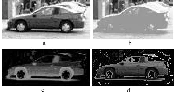
P (i, j)= r, s , (t, v) : I(r, s)=i, I(t, v)= j Fig. 1: a) A sample occluded image with natural
background denoted as I (x, y). b) The small regions are removed by filling the holes. c) Image difference obtained by subtraction (a) by (b) denoted as d (x, y). d) Image obtained by mapping function f (x, y)
BACKGROUND REMOVAL AND MAPPING FUNCTION
The overall complexity increases for the natural images as the object of interest is lying on the background region. In object classification problem, it is essential to distinguish the object of interest and the background. Segmentation of object is done through background subtraction technique. This method is more suitable when the intensity levels of the objects fall outside the range of levels in the background.
An object with natural background is shown in Fig. 1. Initially morphological operations are applied to suppress the residual errors with help of open and close pair statements (Li et al., 2004; Richord et al., 2005). The small regions are removed by filling the holes. Then, the image subtraction is applied with the previous result. Thus, the object is segmented from the background.
A mapping function (1) is used to restore the object of interest from that of the subtracted image.
(1)
where, f (x, y) is the transformed image, d (x, y) is image difference after fill operation and I (x, y) is the original image.
STATISTICAL FEATURES
Statistical functions such as mean, median, standard deviation and higher moments are most common to characterize data set, which have been used as pattern features in many applications (Papageorgiou and Poggio, 1999; Said et al., 2000, 2001). Higher moments can be used to classify the actual shape of the distribution function. Depend on the statistical analysis of the vector, we extract 6 features as follows:
Feature (1): Mean or the average, which is defined as:
(2)
where, is the mean value and N is the total number of data values, x .i
Feature (2): The standard deviation: The best known measure of the spread of the distribution is the simple variance and it is defined as:
(3)
The standard deviation is a well-known measure of deviation from its mean value and is defined as the square root of the variance.
(4)
Feature (3): Smoothness is measured with its second moment as:
(5)
Feature (4): The skewness, or third moment, is a measure of asymmetry of distribution defined as:
(6)
Feature (5): Energy is calculated as:
(7)
The gray level co-occurrence matrix P for ad
displacement vector d= (d , d ) is defined in (8). The entryx y
(I, j) for P is the number of occurrences of the pair of grayd
levels i, j which are a distance d apart.
(8)
[image:2.612.96.273.94.187.2]j i
d d i j
entropy= −
∑∑
P (i, j) log P (i, j)( )
N l 1l l l 1
j jm m
m 0
O k f w O
− − =
=
∑
(9)
It should be noted that spatial gray level co-occurrence estimated image properties are related to the second order statistics of image.
Thus 6 statistical measures of texture are calculated for every sub-block of an image. The feature vector is populated with multiples of 6 with that of number of sub-blocks in an image.
BUILDING A NEURAL CLASSIFIER
A binary Artificial Neural Network (ANN) classifier is built with back-propagation algorithm that learns to classify an image as a member or nonmember of a class.
The number of input layer nodes is equal to the dimension of the feature space obtained from the moments and invariant features. The number of output nodes is usually determined by the application (Khotanzand and Chung, 1998) which is 1 (either Yes/ No) where, a threshold value nearer to 1 represents Yes and a value nearer to 0 represents No. The neural classifier is trained with different choices for the number of hidden layer. The final architecture is chosen with single hidden layer shown in Fig. 2 that results with better performance.
The connections carry the outputs of a layer to the input of the next layer have a weight associated with them. The node outputs are multiplied by these weights before reaching the inputs of the next layer. The output neuron (10) will be representing the existence of a particular class of object.
[image:3.612.297.534.395.690.2](10)
Fig. 2: The 3 layer neural architecture
PROPOSED WORK
This study addresses the issues to classify objects of real-world images containing side views of cars amidst background clutter and mild occlusion. The objects of interest to be classified are car (positive) and non-car (negative) images taken from University of Illinois at Urbana-Champaign (UIUC) standard database. The image data set consists of 1000 real images for training and testing having 500 in each class. The sizes of the images are uniform with the dimension 100×40 pixels.
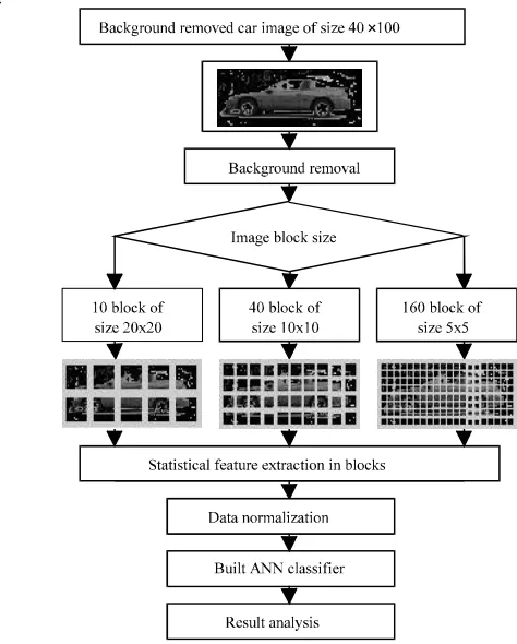
The proposed framework consists of 3 methods followed by background removal as given in section Method-I: 10 Blocks of size 20×20 each, Method-II: 40 Blocks of size 10×10 each Method-III: 160 Blocks of size 5×5 each. Six statistical features are calculated from each single block of sub-image using equations mentioned in section-II. Data normalization is applied for the statistical features, which are the deviated from its mean by standard deviation. This process improves the performance of the neural classifier. The overall flow of the framework is shown in Fig. 3.
[image:3.612.94.272.534.694.2]IMPLEMENTATIONS
We trained our methods with different kinds of cars against a variety of background, partially occluded cars of positive class. The negative training examples include images of natural scenes, buildings and road views. The training is done with 400 images (200 positive and 200 negative) against all the methods. The testing of images are done with 1000 images (500 positive and 500 negative) taken from the same image database.
[image:4.612.331.503.97.269.2]The feed-forward network for learning is done for 10 blocks of size 20×20 namely method-I, 40 blocks of size 10×10 namely method-II and 160 blocks of size 5×5 namely method-III, respectively. The input nodes for method-I is 60 (10 blocks ×6 features), method-II is 240 (40 blocks ×6 features) and method-III is 960 (160 blocks ×6 features), respectively. Optimal structure validation is done and the structure given below performs well and leads to better results. Thus the optimal structure (Fig. 2) of the neural
Fig. 4: The performance graph of neural network training for Method-I: 10 Blocks of size 20×20
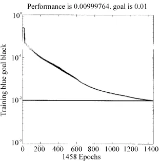
Fig. 5: The performance graph of neural network training
[image:4.612.314.540.318.385.2]for Method-II: 40 Blocks of size 10×10 Rate (FNR).
[image:4.612.94.260.345.498.2]Fig. 6: The performance graph of neural network training for Method-III: 160 Blocks of size 5×5
Table 1: Parameters for training of the neural classifier
Parameters Method-I Method- II Method-III
Learning Rate 0.5 0.5 0.5
Performance Goal 0.01 0.01 0.01
No. of Epochs taken to 12261 1458 368
meet the performance goal
Time taken to learn 141.26 20.64 24.20
Secs Secs Secs
classifier for method-I is 60-20-1, method-II is 240-10-1 and method-III is 960-25-1, respectively.
The various parameters for the neural classifier training for all the methods are given in Table 1. The Performance graph of the neural classifier for method-I method-II and method-III are shown in Fig. 4-6, respectively.
DISCUSSION
In object classification problem, the four quantities of results category are given.
True Positive (TP): Classify a car image into class of cars.
True Negative (TN): Misclassify a car image into class of Non-cars.
False Positive (FP): Classify a non-car image into class of non-cars.
False Negative (FN): Misclassify a non-car image into class of cars.
[image:4.612.100.255.542.699.2]( )
( )
Number of true positive TP TPRTotal number of positive in data set nP =
( )
( )
Number of true negative TN TNRTotal number of negative in data set nN =
( )
( )
Number of false positive FP FPR
Total number of positive in data set nP =
( )
( )
Number of false negative FN FNR
Total number of negative in data set nF =
[image:5.612.85.276.96.191.2]Fig. 7: Sample results of the neural classifier of the category car images with cluttered background and mild occlusion
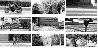
Fig. 8: Sample results of the neural classifier of the category non-car images containing trees, road view, bike, wall, buildings and persons
Table 2: Comparison of experimental methods
Classifying positive Classifying negative images (car images) images (non-car images) Threshold for ---
---Classification: 0.7 TPR TNR FPR FNR
Method-I 78.6% 21.4% 84.4% 15.2%
10 Blocks of Method-I
size 20 × 20 Overall Classification Accuracy (TPR+FPR)/2 is 81.5%
Method-II 78.4% 21.6% 88.4% 11.6%
40 Blocks of Method-II
size 10 × 10 Overall Classification Accuracy (TPR+FPR)/2 is 83.4%
Method-III 74.8% 25.2% 92.8% 7.2%
160 Blocks of Method-III
size 5 × 5 Overall Classification Accuracy (TPR+FPR)/2 is 83.8%
The values of nP and nN used as testing samples are 500 and 500, respectively. Most classification algorithm includes a threshold parameter for classification accuracy which can be varied to lie at different trade-off points between correct and false classification. The comparison of results of the proposed methods is shown in Table 2 which is obtained with an activation threshold value of 0.7.
Classified images of category car and non-car as resultant sample images are shown below in the Fig. 7 and 8, respectively.
It is evident that the classifier with 160 blocks of size 5 × 5 (Method-III) is showing improved overall results of 83.8% of classification accuracy comparatively with that of 40 blocks of size 10 × 10 (Method-II) and 10 blocks of size 20×20 (Method-I). Method-II is also comparatively, good in classification with the accuracy of 83.4%.
CONCLUSION
Thus an attempt is made to build a system that classifies the objects amidst background clutter and mild occlusion is achieved to certain extent. Thus the goal to classify objects of real-world images containing side views of cars with cluttered background with that of non-car images with natural scenes is presented. Comparing the results in Table 2, the performance of the proposed method with 160 blocks of size 5×5 with statistical features after background removal gives a satisfactory classification rate of 83.8%. There by the average classification accuracy is slightly improved by 4.2% compared with the wavelet based method proposed by Nagarajan and Balasubramanie (2007). The limitation of this method is the object with a high degree of occlusion for classification. Further work extension can be made to improve the performance of the classifier system with the inclusion of feature selection process. This complete research is implemented using neural network and image processing toolbox of Matlab 6.5.
REFERENCES
Agarwal, S., A. Awan and D. Roth, 2004. Learning to detect objects in images via a sparse, part-based representation. IEEE. Trans. Pattern Anal. Machine Intell., 26 (11): 1475-1490.
Hsieh, J.W. et al., 2006. Automatic traffic surveillance system for vehicle tracking and classification. IEEE. Trans. Intell. Trans. Syst., 7 (2): 175-187.
[image:5.612.88.276.249.341.2]Li, L. et al., 2004. Statistical modeling of complex Sun, Z. et al., 2006. Monocular precrash vehicle detection: backgrounds for foreground object detection. IEEE.
Trans. Image Proc., 13 (11): 1459-1472.
Nagarajan, B. and P. Balasubramanie, 2007. Wavelet feature based neural classifier system for object classification with complex background. Iccima 07. IEEE Comp. Soc. Press, 1: 302-307.
Papageorgiou, C.P. and T. Poggio, 1999. A trainable object detection system: Car detection in static images. A.I. Memo No. 1673, Massachusetts Institute of Technology: MIT.
Said, E.E. et al., 2000. Neural network face recognition using statistical feature extraction. 17th national radio science conference. Minufiya University, Egypt, C31: 1-8.
Features and classifiers. IEEE. Trans. Image Proc., 15: 2019-2034.
Richord, J.R. et al., 2005. Image change detection algorithms: A systematic survey. IEEE. Trans. Image Proc., 14 (3): 294-306.
Said, E.E. et al., 2001. Neural network face recognition using statistical feature and skin texture parameters. 18th National Radio Science Conference. Mansoura University, Egypt, C5: 1-8.