http://wrap.warwick.ac.uk
Original citation:
Li, Ruizhe, Kotropoulos, Constantine, Li, Chang-Tsun and Guan, Yu (Researcher in
Computer Science) (2015) Random subspace method for aource camera identification.
In: IEEE International Workshop on Machine Learning for Signal Processing (MLSP'15),
Boston, USA, 17-20 Sept 2015. Published in: 2015 IEEE 25th International Workshop on
Machine Learning for Signal Processing (MLSP)
Permanent WRAP url:
http://wrap.warwick.ac.uk/75553
Copyright and reuse:
The Warwick Research Archive Portal (WRAP) makes this work by researchers of the
University of Warwick available open access under the following conditions. Copyright ©
and all moral rights to the version of the paper presented here belong to the individual
author(s) and/or other copyright owners. To the extent reasonable and practicable the
material made available in WRAP has been checked for eligibility before being made
available.
Copies of full items can be used for personal research or study, educational, or not-for
profit purposes without prior permission or charge. Provided that the authors, title and
full bibliographic details are credited, a hyperlink and/or URL is given for the original
metadata page and the content is not changed in any way.
Publisher’s statement:
“© 2015 IEEE. Personal use of this material is permitted. Permission from IEEE must be
obtained for all other uses, in any current or future media, including reprinting
/republishing this material for advertising or promotional purposes, creating new
collective works, for resale or redistribution to servers or lists, or reuse of any
copyrighted component of this work in other works.”
A note on versions:
The version presented here may differ from the published version or, version of record, if
you wish to cite this item you are advised to consult the publisher’s version. Please see
the ‘permanent WRAP url’ above for details on accessing the published version and note
that access may require a subscription.
INCREMENTAL UPDATE OF FEATURE EXTRACTOR FOR CAMERA IDENTIFICATION
Ruizhe Li, Chang-Tsun Li, and Yu Guan
Department of Computer Science, University of Warwick, Coventry, CV4 7AL, UK
ruizhe.li, c-t.li, [email protected]
ABSTRACT
Sensor Pattern Noise (SPN) is an inherent fingerprint of imaging devices, which has been widely used in the tasks of digital camera identification, image classification and forgery detection. In our previous work, a feature extraction method based on PCA denoising concept was applied to extract a set of principal components from the original noise residual. However, this algorithm is inefficient when query cameras are continuously received. To solve this problem, we propose an extension based on Candid Covariance-free Incremental PCA (CCIPCA) and two modifications to incrementally update the feature extractor according to the received cameras. Experi-mental results show that the PCA and CCIPCA based features both outperform their original features on the ROC perfor-mance, and CCIPCA is more efficient on camera updating.
Index Terms— Digital forensics, sensor pattern noise, camera identification, PCA denoising
1. INTRODUCTION
Digital camera identification is the process of linking digital images to the cameras that acquired them. Sensor pattern noise has been proved to be a reliable fingerprint of imaging device for digital camera identification. The deterministic component of SPN is the photo-response nonuniformity (PRNU) noise, which is primarily caused by the variable sensitivity of each sensor pixel to light. It is essentially slight variations in the intensity of individual pixels and an unique pattern deposited in every image taken by a sensor.
To determine whether a query image is taken by a suspect camera, three steps have to be taken. 1) The first step is the SPN extraction from the query image. Lukaset al. [1] first adopted a wavelet-based Wiener filter to extract SPN from digital image. After that several methods for SPN extraction or enhancement have been proposed. Dabovet al. [2] pro-posed a sparse 3D transform-domain collaborative filtering to extract SPN. Since PRNU is a kind of multiplicative noise,
Chenet al.[3] proposed a Maximum Likelihood Estimation
(MLE) method to estimate the corresponding multiplicative factor from the reference images. In [4], Li introduced a SPN enhancer to suppress the contamination caused by image content. A further investigation into SPN’s
location-dependent quality is reported by Li and Satta in [5]. In [6], Li
et al.proposed a Colour-Decoupled PRNU extraction method
to prevent the CFA interpolation noise from propagating into the physical components. In [7], Kanget al.introduced a con-text adaptive SPN predictor to suppress the impact of image content. 2) The second step is to estimate the reference SPN from the suspect camera, usually done by averaging multiple SPNs extracted from smooth images taken by that camera. 3) The final step is to detect whether the query SPN correlates to the suspect camera. Normalized cross-correlation is usually adopted as the detector statistics [1]. Later, Goljanet al.[8] introduced the Peak to Correlation Energy ratio (PCE) as a replacement for the normalized correlation detector. Another detection statistic CCN (correlation over circular correlation norm) is then proposed by Kanget al.[9].
There have been many efforts to improve the performance of digital camera identification. Some aimed at improving accuracy, others aimed at improving efficiency. In real applications, sensor fingerprint is usually extracted from large image blocks, since large image blocks contain more SPN information. However, the complexity of both SPN extraction and correlation detection are proportional to the number of pixels in noise residual. Hence the high dimensionality will make the process of camera identification time consuming. To solve this problem, Goljanet al.[10] proposed a fingerprint digest, which is formed by keeping only a small number of the largest fingerprint values and their positions. Later, Huet al.[11] proposed a fast fingerprint digest search algorithm to further improve the identification efficiency. In [12], Bayram
et al. proposed to represent sensor fingerprint in
binary-quantized form, which speeds-up the correlation detection and also greatly reduce the size of fingerprint.
2. PROPOSED METHOD
2.1. PCA-based feature extraction
In SPN based camera identification, we usually extract noise residual from large image blocks to improve the identifica-tion accuracy, since large image blocks contain more SPN information. As a result, noise residual usually has a very high dimensionality (e.g. 1024×1024 pixels). However, the high-dimensional noise residual also tends to contain more redundancy and interfering components. For example, noise residual can be contaminated by color interpolation, JPEG compression, distortion introduced by denoising filter and other artifacts. Most of these artifacts are non-unique, redun-dant and less discriminant. Removing them will enhance the SPN signal in noise residual and improve the identification accuracy. Nevertheless, they are mixed with the real SPN signal in noise residual and it is very hard to separate them.
PCA [15] is a decorrelation method which has been widely used for dimensionality reduction and redundancy removal. In our case, we attempt to find a PCA transformed domain which can better separate the real SPN signal and these redundant features. By excluding these redundant features, we can extract a set of features which contain most of the discriminative information of SPN signal.
2.1.1. Optimization of training samples
However, SPN is a subtle signal which can be severely contaminated in noise residual by scene details. These scene details may significantly increase the number of irrelevant components. And these components will be more dominant than SPN signal. Without removing these strong contamina-tions from the training set, PCA is more likely to find a set of components that will represent these noisy components rather than the real SPN signal. To avoid this problem, two strategies are applied:
1) Sample selection. For training sample selection, we
give the priority to the noise residual extracted from low-variation images. It is because such images are more close to the evenly lit scene and contain less scene details. Hence these images can better exhibit the changes caused by SPN in intensity between individual pixels. By choosing this kind of images for SPN extraction, it will capture the energy of true SPN in the training set and guide PCA to find a set of features that better represent the SPN signal rather than other noisy components.
2) SPN extraction.Several SPN extraction methods in the literature could be used here to further enhance the energy of SPN signal in training set. Note that this step would be more important when only natural images (with scene details) instead of low-variation images are available for training. Assume there are n images {Ii}ni=1 taken by c cameras
{Cj}cj=1in the database. We first extract noise residual from
theN×N-pixels blocks cropped from the centre of these full-sized images and reshape them into a set of column vectors
{xi ∈RN2×1}ni=1with zero mean. ThesenSPN vectors are then used as the training set.
2.1.2. PCA-based extractor and limitation
PCA is performed to seek a set of orthonormal vectorsvkand their associated eigenvaluesλk. The vectorsvk and scalars
λk are the eigenvectors and eigenvalues, respectively, of the covariance matrixS
S= 1
n
n
∑
i=1
xixTi =AAT (1)
whereA=√1
n[x1, . . . ,xn]∈R N2×n
. Notice that the dimen-sionality of SPN could be extremely high (e.g.,N2=10242).
Therefore, directly solving the eigenvalue decomposition problem ofS ∈RN2×N2 incurs a prohibitive computational cost (with a complexityO(N6)). To make PCA feasible for the high-dimensional SPN, we apply a fast method instead of computing these eigenvectors (whenn≪N2). Assumev
k′ is the unit eigenvector ofATA∈ Rn×n with eigenvalueλ′
k. We could obtainATAv
k′ =λk′vk′. Multiplying both sides byA, we haveAAT(Av
k′) = λk′(Avk′), whereAvk′ are the eigenvectors ofAAT = S with eigenvaluesλ
k′. Thus, instead of solving the eigenvalue decomposition of matrix
S directly, we can calculate the eigenvectors vk′ via the smaller matrixATA∈Rn×n and obtain the objectivevk by vk =Avk′. The obtained{vk}n
k=1are then normalized and
sorted in the descending order according to their associated eigenvaluesλ1≥λ2≥...λn. Note that only whenn≪N2, computing eigenvectors via this method (with a complexity
O(n3)) would be more effective than the traditional way. The eigenvectors with thedlargest eigenvalues are select-ed to form a feature extractor M = [v1, ...,vd] ∈ RN
2×d
. We keep the topdeigenvectors corresponding to99%of the variance as it could give us the best result. Based on this feature extractorM, we can obtain a new feature with much lower dimensionality by
yi=MTxi, i= 1,2, ..., n. (2)
whereyi∈Rd×1is the compact version of the original vector xi. The experimental results in Section 3 show that this PCA-based feature could outperform its original feature according to the ROC analysis, which means the SPN signal has been further purified during this feature extraction.
2.2. Incremental camera learning
Incremental learning method is usually adopted to add new samples to the original training set and update the PCA representation with less computational burden. CCIPCA was introduced in [16] to incrementally update the leading eigenvectors without estimating the covariance matrix. In this work, we propose a method based on CCIPCA to incremen-tally update feature extractor so as to accommodate the new received images/cameras. Assume we have already computed the initial feature extractorM from the original training set
{xi}n
i=1. We can generatenˆ noise residual vectors{xiˆ}niˆ=1
from the continuously receivedcˆcameras. To incrementally update the feature extractor according to these new cameras, we can use the following algorithm
Algorithm
Input:The initial feature extractorM = [v0
1,v20, ...,v0d], the new received SPN vectors{xiˆ ∈RN2×1}ˆn
i=1fromˆccameras;
Output: The new feature extractor Mˆ = [vn1ˆ,vn2ˆ, ...,vdnˆˆ]
updated bynˆsamples;
fori= 1toˆndo
step 1:v0
d+i =
ˆ xi
∥xˆi∥,M=[v
0
1,v02, ...,vd0+i]∈RN
2×(d+i)
;
step 2: Initializingxˆ1 i =xiˆ;
fork= 1tod+ido
step 3:vi k =
n−l−1 n v
i−1 k +
l+1 n xˆ
k ixˆkTi
vki−1 ∥vki−1∥;
step 4:xˆki+1=xˆk i −xˆkTi
vki ∥vi k∥
vki ∥vi k∥
;
end for end for
step 5: After normalizing[vnˆ
1,v2nˆ, ...,vdnˆ+i], selecting the first
ˆ
dleading eigenvectors to form a new feature extractorMˆ = [vnˆ
1,v2ˆn, ...,vdˆnˆ]∈R N2×dˆ
.
In this algorithm,vi
kis thek-th eigenvector derived from the first receivedisample vectors. xˆki+1means the residual of the samplexˆiafter subtracted by the projections in the first
keigenvectors[vi
1,vi2, ...,vik], and serves as the input data for the next iteration. By doing so, the residual left by the firstk
eigenvectors will be complemented in the computation of the higher order eigenvectors.
Compare to the algorithm in [16], the main contributions of our method are: 1) step 1 is introduced in this algorithm to support more eigenvector candidates for constructing the new feature extractorMˆ, which could improve the accuracy of extractor estimation for accommodating the new cameras. At the meantime, step 5 is proposed to keep the extractor low dimensionality by discarding the less important eigenvectors from all the candidates. 2)lis the weighting parameter. We run this algorithm withl=−0.8to prevent from assigning too much weight to the new cameras and diluting the effect of old cameras. For each new arrived sample, the direction of every eigenvector will be adjusted once. To avoid too much adjustment for a signal camera, we use at maximum 5 samples from each newly received camera for updating.
3. EXPERIMENTS
3.1. Experimental setup
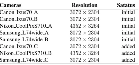
In this work, the noise residuals extracted by the methods in [3] (MLE) and [7] (Kang) are used as the original features. In order to testify the feasibility of the proposed method, the performance of these original features combined with and without the proposed scheme are compared. The experimen-tal work are conducted over the Dresden Image Database [17]. A total of 1600 images from 8 cameras are involved in our experiments, each responsible for 200. These 8 cameras belong to 3 camera models, each camera model has 2∼3 different devices. These cameras are listed in Table 1. For each camera, we have 50 low-variation images for training and 150 images with scene details for testing. Hence there are
150×8matching and1050×8mismatching pairs in total. In our experiments, MLE/Kang+8C-PCA indicates that all the noise residual are extracted by MLE/Kang method and the feature extractor is estimated by PCA which includes all the 8 cameras in the training process; 5C-PCA means only the 5 initial-cameras are involved in PCA training; and 5(3)C-CCIPCA denotes that the 5initial-cameras are first applied by PCA to estimate the initial feature extractor and the rest
3 added-cameras are then sequentially added to update the
[image:4.595.55.297.252.464.2]initial feature extractor via our CCIPCA-based method.
Table 1. Cameras from Dresden Database
Cameras Resolution Satatus
Canon Ixus70 A 3072×2304 initial
Canon Ixus70 B 3072×2304 initial
Nikon CoolPixS710 A 4352×3264 initial
Samsung L74wide A 3072×2304 initial
Samsung L74wide B 3072×2304 initial
Canon Ixus70 C 3072×2304 added
Nikon CoolPixS710 B 4352×3264 added
Samsung L74wide C 3072×2304 added
3.2. Performance evaluation
Fig.1 shows the histograms of correlation values obtained from different methods. By comparing Fig. 1(a) with Fig. 1(b) and 1(c), we can see that after the feature extraction, the separation between intraclass and interclass is clearer and the overlapping area becomes smaller. It suggests that the features extracted by 8C-PCA or 5(3)C-CCIPCA are both superior than their original feature. But the performance of 8C-PCA is the upper bound of 5(3)C-CCIPCA. Such as in Fig. 1(c), we can see the tail of the mismatching distribution is wider than that in Fig. 1(b). This is mainly due to the approximation error between the principal components of PCA and those of CCIPCA. However, so far it still remains anopen questionand beyond the scope of this paper.
[image:4.595.316.560.389.503.2]Correlation
-0.05 0 0.05 0.1 0.15
Count
0 100 200 300 400 500
Mismatching Matching
(a) Histograms for MLE method
Correlation
-0.4 -0.2 0 0.2 0.4 0.6 0.8 1
Count
0 100 200 300 400 500
Mismatching Matching
(b) Histograms for MLE + 8C-PCA
Correaltion
-0.4 -0.2 0 0.2 0.4 0.6 0.8 1
Count
0 100 200 300 400 500
Mismatching Matching
(c) Histograms for MLE + 5(3)C-CCIPCA
Fig. 1. Histogram for the correlation values obtained from different methods,256×256pixels (Note the X-axis range).
False positive rate
0 0.1 0.2 0.3 0.4 0.5 0.6 0.7 0.8 0.9 1
True positive rate
0.8 0.82 0.84 0.86 0.88 0.9 0.92 0.94 0.96 0.98
1 Overall ROC curves, 256x256 pixels
MLE+5C-PCA MLE
MLE+5(3)C-CCIPCA MLE+8C-PCA
Fig. 2. ROC curves of different features based on MLE [3].
False positive rate
0 0.1 0.2 0.3 0.4 0.5 0.6 0.7 0.8 0.9 1
True positive rate
0.8 0.82 0.84 0.86 0.88 0.9 0.92 0.94 0.96 0.98
1 Overall ROC curves, 256x256 pixels
Kang+5C-PCA Kang
Kang+5(3)C-CCIPCA Kang+8C-PCA
Fig. 3. ROC curves of different features based on Kang [9].
can see that: 1) The ROC performance of features extracted by 8C-PCA and 5(3)C-CCIPCA are both higher than that of the original features. It is because that the proposed feature extractor can further exclude the redundancy and interfering features from the noise residual obtained by the MLE or Kang method. 2) The ROC performance of 5C-PCA is the worst among the four methods. This is mainly because that this feature extractor is only estimated from the 5 initial -cameras, which is not accurate enough to represent the rest
3 added-cameras. Thus, there will be a large number of
false positives from these 3 added-cameras. Repeating a training that includes these 3added-cameras can regain the
Table 2. Computational time for updating a single camera to
a training set with 10, 20 and 40 cameras, respectively. Training time (Seconds)
10+1 cameras 20+1 cameras 40+1 cameras
PCA 2.91 9.65 45.84
CCIPCA 0.85 0.86 0.86
accuracy, but it will incur costly re-computation especially when the number of overall cameras is huge. Therefore, our CCIPCA-based method is proposed to improve the efficiency. We can see from Table 2, the computational time can be significantly reduced by applying CCIPCA to update new cameras. 3) The ROC performance of 5(3)C-CCIPCA feature is very close to that of 8C-PCA. This is a good indication that the proposed incremental updating approach can not only significantly improve the updating efficiency, but also well preserve the identification accuracy.
4. CONCLUSION
[image:5.595.87.529.77.200.2] [image:5.595.65.282.227.379.2] [image:5.595.65.280.403.557.2]5. REFERENCES
[1] J. Lukas, J. Fridrich, and M. Goljan, “Digital camera identification from sensor pattern noise,” IEEE Trans. Inf. Forensics Security, vol. 1, no. 2, pp. 205–214, 2006.
[2] K. Dabov, A. Foi, V. Katkovnik, and K. Egiazarian, “Image denoising by sparse 3d transform-domain col-laborative filtering,” IEEE Trans. Image Process., vol. 16, no. 8, pp. 2080–2095, 2007.
[3] M. Chen, J. Fridrich, M. Goljan, and J. Lukas, “Deter-mining image origin and integrity using sensor noise,”
IEEE Trans. Inf. Forensics Security, vol. 3, no. 1, pp. 74–90, 2008.
[4] C.-T. Li, “Source camera identification using enhanced sensor pattern noise,” IEEE Trans. Inf. Forensics Security, vol. 5, no. 2, pp. 280–287, 2010.
[5] C.-T. Li and R. Satta, “Empirical investigation into the correlation between vignetting effect and the quality of sensor pattern noise,” IET Computer Vision, vol. 6, no. 6, pp. 560–566, 2012.
[6] C.-T. Li and Y. Li, “Color-decoupled photo response non-uniformity for digital image forensics,” IEEE Trans. Circuits Syst. Video Technol., vol. 22, no. 2, pp. 260–271, 2012.
[7] X. Kang, J. Chen, K. Lin, and A. Peng, “A context-adaptive spn predictor for trustworthy source camera identification,” EURASIP Journal on Image and Video Processing, vol. 2014, no. 1, pp. 1–11, 2014.
[8] M. Goljan, “Digital camera identification from images - estimating false acceptance probability,” inProc. of International Workshop on Digital-forensics and Water-marking, pp. 454–468. 2009.
[9] X. Kang, Y. Li, Z. Qu, and J. Huang, “Enhancing source camera identification performance with a camera reference phase sensor pattern noise,” IEEE Trans. Inf. Forensics Security, vol. 7, no. 2, pp. 393–402, 2012.
[10] M. Goljan, J. Fridrich, and T. Filler, “Managing a large database of camera fingerprints,” inProc. SPIE, Electronic Imaging, Media Forensics and Security XII, San Jose, CA, USA, Jan. 17C21, 2010, vol. 7541, pp. 08 01–12.
[11] Y. Hu, C.-T. Li, and Z. Lai, “Fast source camera identification using matching signs between query and reference fingerprints,” Multimedia Tools and Applica-tions, pp. 1–24, 2014.
[12] S. Bayram, H. Sencar, and N. Memon, “Efficient sensor fingerprint matching through fingerprint binarization,”
IEEE Trans. Inf. Forensics Security, vol. 7, no. 4, pp. 1404–1413, 2012.
[13] D. Zhang, R. Lukac, X. Wu, and D. Zhang, “PCA-based spatially adaptive denoising of CFA images for single-sensor digital cameras,” IEEE Trans. Image Process., vol. 18, no. 4, pp. 797–812, 2009.
[14] R. Li, C.-T. Li, and Y. Guan, “A compact representation of sensor fingerprint for camera identification and fin-gerprint matching,” in Proc. IEEE International
Con-ference on Acoustics, Speech, and Signal Processing,
Brisbane, Australia, Apr. 19-24, 2015.
[15] K. Fukunaga, Introduction to Statistical Pattern
Recog-nition, 2nd ed. New York: Academic, 1991.
[16] J. Weng, Y. Zhang, and W.S. Hwang, “Candid covariance-free incremental principal component anal-ysis,” IEEE Trans. Pattern Anal. Mach. Intell., vol. 25, no. 8, pp. 1034–1040, 2003.