warwick.ac.uk/lib-publications
A Thesis Submitted for the Degree of PhD at the University of Warwick
Permanent WRAP URL:
http://wrap.warwick.ac.uk/99207
Copyright and reuse:
This thesis is made available online and is protected by original copyright.
Please scroll down to view the document itself.
Please refer to the repository record for this item for information to help you to cite it.
Our policy information is available from the repository home page.
U N
IV
ER
SITAS WARWICEN SIS
Mining Previously Unknown Patterns in Time
Series Data
by
Zhuoer Gu
A thesis submitted to The University of Warwick
in partial fulfilment of the requirements
for admission to the degree of
Doctor of Philosophy
Department of Computer Science
The University of Warwick
The emerging importance of distributed computing systems raises the needs of
gaining a better understanding of system performance. As a major indicator of
system performance, analysing CPU host load helps evaluate system performance
in many ways. Discovering similar patterns in CPU host load is very useful since
many applications rely on the pattern mined from the CPU host load, such as
pattern-based prediction, classification and relative rule mining of CPU host
load.
Essentially, the problem of mining patterns in CPU host load is mining
the time series data. Due to the complexity of the problem, many traditional
mining techniques for time series data are not suitable anymore. Comparing
to mining known patterns in time series, mining unknown patterns is a much
more challenging task. In this thesis, we investigate the major difficulties of the
problem and develop the techniques for mining unknown patterns by extending
the traditional techniques of mining the known patterns.
In this thesis, we develop two different CPU host load discovery methods:
the segment-based method and the reduction-based method to optimize the
pattern discovery process. The segment-based method works by extracting
segment features while the reduction-based method works by reducing the size
of raw data. The segment-based pattern discovery method maps the CPU host
load segments to a 5-dimension space, then applies the DBSCAN clustering
method to discover similar segments. The reduction-based method reduces
The investigations into the CPU host load data inspired us to further develop
a pattern mining algorithm for general time series data. The method filters out
the unlikely starting positions for reoccurring patterns at the early stage and
then iteratively locates all best-matching patterns. The results obtained by our
method do not contain any meaningless patterns, which has been a different
problematic issue for a long time. Comparing to the state of art techniques, our
Biggest thanks and gratitude go to my supervisor Dr. Ligang He, without whom
I would not have had the change to pursuing my research. His guidance will
always be my invaluable treasure.
Sincere thanks to my parents. It is their selfless care, support, and love that
make me who I am today.
Thanks to my fantastic lab-mates, Bo Gao, Chao Chen, Huanzhou Zhu,
Shenyuan Ren, Pengjiang, Junyu Li, Bo Wang, Mohammed Alghamdi and
Nentawe Gurumdimma who I shared fantastic time with. It has been a great
pleasure to work with them.
Special thanks to rainy Tocil Wood for teaching me a lesson that a tempting
path sometimes leads to nowhere, and you better head back before your shoes
Parts of this thesis have been previously published by the author in the following:
• Z. Gu, C. Chang, L. He, and K. Li. Developing a pattern discovery model
for host load data. InComputational Science and Engineering (CSE), 2014
IEEE 17th International Conference on, pages 265–271. IEEE, 2014
• Z. Gu, L. He, C. Chang, J. Sun, H. Chen, and C. Huang. An efficient
method for motif discovery in cpu host load. In Fuzzy Systems and
Knowledge Discovery (FSKD), 2015 12th International Conference on,
pages 1027–1034. IEEE, 2015
• Z. Gu, L. He, C. Chang, J. Sun, H. Chen, and C. Huang. Developing
an efficient pattern discovery method for cpu utilizations of computers.
International Journal of Parallel Programming, pages 1–26, 2016. ISSN
1573-7640. doi: 10.1007/s10766-016-0439-0. URLhttp://dx.doi.org/ 10.1007/s10766-016-0439-0
• S. Ren, L. He, H. Zhu, Z. Gu, W. Song, and J. Shang. Developing
power-aware scheduling mechanisms for computing systems virtualized by xen.
Concurrency and Computation: Practice and Experience, 29(3), 2017
In addition, the following works are either in progress:
• (Unsubmitted) Segmentation Clustering Based CPU Host Load Pattern
CPU Central Processing Unit
DTW Dynamic Time Warping
DDTW Derivative Dynamic Time Warping
PAA Piecewise Aggregative Approximation
SAX Symbolic Aggregative approXimation
ASPL Approximate Similar Pattern Locating
AR AutoregRessive model
MA Moving Average model
ARMA AutoregRessive Moving Average model
ARIMA AutoRegressive Integrated Moving Average model
ARFIMA AutoRegressive Fractionally Integrated Moving Average model
HMM Hidden Markov Model
DFT Discrete Fourier Transform
DWT Discrete Wavelet Transform
LCSS Longest Common SubSequence
ECG Electrocardiograph
VM Virtual Machine
HPC High Performance Computing
PSR Phase Space Reconstruction
SVD Singular Value Decomposition
SAM Spatial Access Method
Abstract ii
Dedication iv
Acknowledgements v
Declarations vi
Sponsorship and Grants viii
Abbreviations ix
List of Figures xv
List of Tables xvi
1 Introduction 1
1.1 CPU Host Load, CPU Host Load Analysing, and Time Series
Unknown Pattern Discovery . . . 3
1.2 Challenges of Pattern Discovery in Time Series Data and CPU
Host Load . . . 5
1.3 Pattern Discovery in CPU Host Load and Time Series: Our
Contributions . . . 10
2.2 CPU Host Load Analysis . . . 16
2.2.1 Statistical Features of CPU Host Load . . . 16
2.2.2 Mining and Prediction of CPU Host Load . . . 18
2.3 Time Series Data Mining Techniques . . . 19
2.3.1 Similarity Measure . . . 19
2.3.2 Time Series Segmentation . . . 22
2.3.3 Time Series Data Representation . . . 24
2.3.4 Time Series Data Indexing . . . 26
2.3.5 Time Series Clustering . . . 27
2.3.6 Similar Pattern Locating in Time Series Data . . . 30
2.4 Summary . . . 31
3 Problem Formalisation 33 3.1 Definitions . . . 33
3.2 Similarity measure . . . 35
3.2.1 Euclidean Distance . . . 35
3.2.2 Dynamic Time Warping and Warping Path Constraint . . 35
3.3 The Similarity Inconsistency Problem . . . 37
3.3.1 Similarity Inconsistency in Original Space . . . 38
3.3.2 Consistent Similarity Measure . . . 40
3.4 Noise Reduction of CPU host load . . . 41
4 Clustering Based CPU Host Load Similar Pattern Discovery 43 4.1 Segmentation Based Data Representation . . . 44
4.1.1 Noise reduction . . . 44
4.1.2 Segmentation . . . 44
4.1.3 Feature Extraction . . . 46
4.2 Pattern Discovery by Clustering . . . 48
4.3.2 The Choice of Parameters . . . 53
4.3.3 Effectiveness of Distance Measure . . . 56
4.4 Summary . . . 57
5 Reduction Based CPU Host Load Pattern Discovery 59 5.1 CPU Host Load Representation . . . 60
5.1.1 Overview of PAA . . . 60
5.1.2 Overview of SAX . . . 62
5.1.3 The Refined Symbolic Aggregate Approximation Indexing 62 5.2 Similarity Measure . . . 65
5.3 Efficient Pattern Discovery . . . 68
5.3.1 Brute Force Pattern Discovery . . . 68
5.3.2 Improved Pattern Discovery Algorithm . . . 69
5.3.3 Cascade Pattern Discovery . . . 70
5.4 Experimental Evaluation . . . 72
5.4.1 Mining patterns in Google Cluster Trace . . . 73
5.4.2 Efficiency of Indexing . . . 73
5.4.3 Efficiency of Pattern Discovery . . . 78
5.5 Summary . . . 80
6 Iterative Similar Pattern Discovery in Time Series Data 82 6.1 Creating Prior Knowledge for Patterns . . . 83
6.2 Approximate Similar Pattern Position Locating . . . 85
6.2.1 Naive Pattern Position Locating . . . 85
6.2.2 Search Space Reduction . . . 87
6.2.3 Invalid Results Reduction . . . 89
6.3 Similar Pattern Discovery Based on Possible Starting Points . . . 91
6.3.1 Naive Similar Pattern Discovery . . . 91
6.4.2 Performance . . . 103
6.5 Summary . . . 107
7 Conclusions and further work 108 7.1 Clustering Based CPU Host Load Pattern Discovery . . . 109
7.2 Reduction Based CPU Host Load Pattern Discovery . . . 110
7.3 Iterative Pattern Discovery of Time Series Data . . . 111
7.4 Further Work . . . 112
1.1 Similar pattern discovery in two CPU host load . . . 5
1.2 Four types of meaningless similar subsequences . . . 7
1.3 Example of similarity inconsistency . . . 8
1.4 Illustration of Gaussian filter retaining the tread of raw data . . 9
1.5 Illustration of noise impact . . . 11
1.6 The effect of noise on distance measure and effectiveness of Gaus-sian filter . . . 12
2.1 A hierarchy of time series representations in the literature . . . . 24
3.1 Illustration of DTW distance . . . 38
3.2 Demonstration of similarity inconsistency . . . 39
4.1 Physical meaning of feature vector . . . 47
4.2 Typical cluster results ofk-means clustering . . . 52
4.3 Typical cluster results of top-down hierarchical clustering . . . . 53
4.4 Typical cluster results of DBSCAN clustering . . . 54
4.5 Left: bottom-up hierarchical clustering result using our proposed distance measure. Right: bottom-up hierarchical clustering result using dynamic time warping. . . 57
5.4 Patterns discovered using host loadaas reference . . . 74
5.5 Indexing efficiency of three indexing methods with dimensional reduce rate of 10 . . . 75
5.6 The proportional relation of efficiency between three indexing methods with different dimensional reduction rates . . . 77
5.7 The time spent by the two algorithms with different data sizes . 78 5.8 Time spent of cascade mining method under different patameter set 79 6.1 A visualization of algorithm 5 and 6 . . . 86
6.2 A visualization of algorithm 7 . . . 93
6.3 Cost matrix and local cost matrix of two example time series . . 94
6.4 Illustration of algorithm 8 . . . 95
6.5 A visualization of algorithm 9 . . . 97
6.6 Pattern discovery on inserted pattern dataset . . . 100
6.7 Pattern discovery on RandomSines dataset . . . 101
6.8 Pattern discovery on Web dataset . . . 101
6.9 Pattern discovery on temperature dataset . . . 102
6.10 Pattern discovery on CPU host load dataset . . . 102
6.11 Pattern discovery on ECG dataset . . . 103
6.12 Runtime of CrossMatch and our method on different datasets . . 104
6.13 Memory consumption of CrossMatch and our method on different datasets . . . 105
6.14 Runtime comparison between CrossMatch and our method as a function of dataset size . . . 106
3.1 Distance of figure 1.3 case under our proposed consistent distance
measure . . . 41
4.1 Average Inner-cluster DTW Distance . . . 55
4.2 Average Inter-cluster DTW Distance . . . 55
5.1 Example of symbol distance look up table . . . 66
6.1 Example of time series grouping compare . . . 87
Introduction
The last decade has been witnessing great changes in computing systems which
are gaining variety, availability, and performance rapidly. Types of computing
systems are now ranging from wearable and mobile devices like smartphones
and smartwatches to publicly available distributed computing systems such as
cloud platforms and clusters. Meanwhile, with the prevalence of mobile devices
and more accessible internet services, applications now tend to offload their
computations and even store data to servers. Cloud services are prevailing for
its cross-platform and device independent features due to the accessibility from
remote ends, despite the devices the clients are using.
Though the performance of modern computing systems is enhanced
exponen-tially on every aspect, the demands on these systems are also increased greatly
and the requirements to these systems are changed in many ways as well. With
a larger number and wider range of people employing local or remote computing
systems, the needs of exploiting potential from computing systems are gathering
consistent attention.
We focus on mining unknown patterns in CPU host load of cluster computing
system, which plays an important role in today’s real-world applications. Much
research has been conducted to enhance the performance of single machines,
per-formance is analysing the features in the host load. In [43], Peter A. Dinda
defined the host load as the number of processes that are running or ready to
run. Later in [42], CPU host is the ratio of total time a CPU is occupied to the
measurement period. We adopt the latter definition as it matches with common
CPU usage measure method and intuitively more comprehensible.
Time series data are ubiquitous in the real world. Unlike static data that
mainly concern the values of the data, time series data are collected with time
and concern both values and changes of the data. The presence of time series
data ranges from stock market price chart to ECG, covers almost every aspect
of human activity. Not only a large portion of data collected in human history
is time series data, many static data mining problems can also be converted to
mining time series data to improve their efficiency or accuracy [155]. Therefore,
mining patterns in time series data is a more general and applicable task and
therefore, it has more potential value.
CPU host load is essentially time series data. Mining unknown patterns in
CPU host load closely relates to mining unknown patterns in time series data.
On the contrary, investigating pattern discovery in time series data helps many
time series pattern related applications including mining CPU host load. We
extend our interest to discover unknown patterns in time series data in later
part of this thesis. Though our work on mining CPU host load data can be
transferred to mining time series data with almost no effort, it is believed that
investigating time series pattern discovery has more significance.
The objectives of this thesis are two folds: we develop methods for mining
unknown patterns in CPU host load and propose novel methods for discovering
unknown patterns in time series data. In this chapter, we first introduce the
problem of mining unknown patterns in CPU host load data, then we extend
the discussion to time series data to reveal the necessity and difficulties of the
1.1
CPU Host Load, CPU Host Load Analysing,
and Time Series Unknown Pattern
Discov-ery
As the major (if not the only) component that handles all the calculation, the
performance and usage of CPUs determine the performance of a computing
system to a great extent. In modern computing systems, performance evaluations
which partly rely on evaluating and estimating performance and usage of CPUs in
these systems are necessary for many applications. According to [8], performance
modelling has at least 4 applications:
1. System design. Systems designs vary when dealing with different types of
load, and distinguish these types often requires locating patterns in system
load.
2. System tuning. System load often involves different patterns which include
periodical subsequences, chaotic subsequences, and smooth subsequences.
In many cases, the occurrences of these subsequences are related in some
way. To analyse the relation to respond accordingly, pattern discovery
should be done in the first place.
3. Application tuning. Different applications bring different effects on the
system’s load, and these effects are likely to be in several different categories.
Analysing these patterns which are brought to CPU load can help gaining
performance for these applications.
4. System procurement. Analysing patterns in CPU host load helps to
understand the needs for a computing system which aids procuring systems
accordingly.
These applications all involve analysing and estimating CPU performance,
which depends on analysing CPU host load of the system. Existing work on
and predicting CPU host load [41, 160]. The result can be useful for
guid-ing schedulguid-ing strategies to achieve high application performance and efficient
resource use [160].
However, locating patterns in CPU host load is less investigated. Discovery
of unknown patterns in CPU host load is the task that finds the start and
end positions of CPU host load subsequences that the two fond subsequences
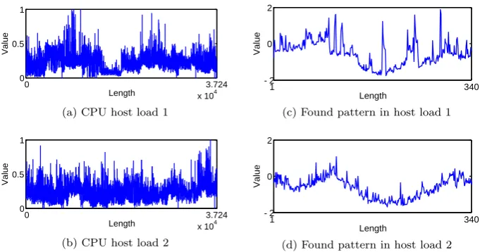
are similar. Figure 1.1 is an example of CPU host load pattern discovery. It
is very useful to discover unknown repeated patterns in CPU host load of a
computing system. Essentially, the CPU host load is time series data [60]. Many
applications rely on pattern discovery in time series data [32], including:
1. The algorithms for mining association rules in time series data based on
pattern discovery [38, 74].
2. Classification algorithms that are based on building typical prototypes of
each class [70, 90].
3. Anomaly detection [39].
4. Finding periodic patterns [66].
Specifically, these applications of mining time series can easily find their
counterparts in mining CPU host load. The use of mining patterns in CPU host
load of a computing system includes but not limited to performance evaluation,
system tuning, job and task scheduling, power usage optimization, fault detection
and respond, CPU host load prediction and users’ using habit mining etc.
Time series data, include CPU host load data, are ubiquitous. As mentioned
previously, mining patterns in time series data is the subroutine of many
real-world time series data mining applications. In bioinformatics, DNA can be
regarded as time series data [9]. Patterns in DNA are often related to genes,
which dominates organisms’ characters. In astronomy, mined patterns from stars’
light intensity changes are used to classify these stars. In medical science, locating
Value
x 104 1
0.5
0
0 3.724
Length
(a) CPU host load 1
Value
x 104 1
0.5
0
0 3.724
Length
(b) CPU host load 2
Value 2 Length 2 0 - 1 340
(c) Found pattern in host load 1
Value 2 Length 2 0 - 1 340
[image:22.595.125.466.124.303.2](d) Found pattern in host load 2
Figure 1.1: Similar pattern discovery in two CPU host load
ECG data. By mining regularity of location information series generated by a
smartphone user, a recommendation system is able to push accurate and useful
information such as traffic information or weather information to the user.
Locating patterns in time series data has attracted a lot of attention. However,
most of these existing work either require a predefined pattern and reduce the
problem to the time series indexing problem, or computationally expensive.
In reality, it is almost impossible for a domain expert to find all the patterns
in a large dataset by experience. Moreover, there exist some patterns which
are beyond the experts’ knowledge. Therefore, an algorithm is needed to find
unknown patterns automatically and efficiently. The algorithm should not require
either the prior knowledge of the length or shape of patterns.
1.2
Challenges of Pattern Discovery in Time
Se-ries Data and CPU Host Load
Comparing to mining patterns in CPU host load data, mining patterns in time
series data is a more general problem and, if there is such a method that can
discover unknown patterns in time series data, we can modify and apply it to
mining tasks reduce to the tasks of mining time series data. These tasks often
relate to locating known patterns in time series data or discovering common
subsequences, or unknown patterns in time series data. Locating known patterns
in time series data has drawn much attention in the last decades and the problem
has been solved in many ways [2, 28, 57, 79]. However, the problem of discovering
previously unknown patterns in time series database remains less focused.
As mentioned in [108] and [32], many applications rely on discovery of
unknown patterns in time series data. In these applications, the task of locating
unknown patterns in time series data reduces to the basic problem of discovering
longest common subsequence pairs, also known as patterns, in two time series
data. Figure 1.1 illustrates the problem intuitively, figure 1.1c and figure 1.1d
are a pair of similar patterns found in time series 1 and time series 2 respectively.
Given the needs and importance of mining previously unknown patterns in
time series data, an obvious method is using nested loops to compare all possible
time series subsequences and find out those similar pairs. However, the time
complexity of this brute force algorithm is as high asO(n6) [60, 62]. Though
optimized by several methods [108], the approach is still unacceptable for mining
patterns on large datasets. The reasons for the high complexity of a naive
method should be owing to the fact that we do not have advance knowledge of
the pattern we are to discover. Specifically, they are:
1. Position of the pattern. If we are able to acknowledge the positions or
possible positions of patterns, the similarity measure can only be performed
on these positions to find out whether they are similar to avoid unnecessary
computation.
2. Length of the pattern. With the knowledge of pattern length, we can
also increase mining efficiency greatly by removing those longer or shorter
candidate subsequences from search space.
3. Shape of the pattern. If the shape of the pattern is known, the problem
has been solved in many ways.
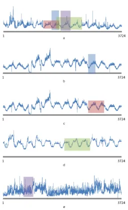
The brute force method also produces a large number of meaningless results.
Figure 1.2 illustrates four typical meaningless results. Figure 1.2a,1.2b and 1.2c
illustrate subsequences pairs that have relatively low distance value but are not
intuitively similar, and figure 1.2d shows one subsequence (blue) is similar to
two subsequences (red) from almost same positions of a time series. For the
brute force method, picking out useful and accurate results from all results is
even a more difficult task.
Value Length 3 2 1 0 -1 1 100
(a) Short similar subsequences
Value Length 3 2 1 0 -1 1 300
(b) Similar subsequences with extreme lengths differnence Value Length 3 2 1 0 -1 1 300
(c) Over-warped similar subsequences
Value Length 3 2 1 0 -1 1 300
[image:24.595.123.464.292.614.2](d) Trivial matches
Figure 1.2: Four types of meaningless similar subsequences
Another problem of finding patterns with arbitrary lengths of is that most
similarity measures are no longer practicable. For example, the two most
commonly used distance measures, Euclidean distance and Dynamic Time
of time series being compared and lower distance value for the shorter pair of
time series being compared. We use a simple experiment to show the effect of
similarity bias as in figure 1.3.
V al u e V al ue V al u e TS128' TS128 TS32' TS32
Length Length
Length
2.5 2.5
2 2
1.5 1.5
1 1
0.5 0.5 TS64'
TS64
0 0
1 128 1 64
2.5 2 1.5 1 0.5 0 1 32
Length 128 64 32
Euclidean 4.20 2.80 1.89
[image:25.595.125.473.196.445.2]DTW 2.10 1.45 1.15
Figure 1.3: Example of similarity inconsistency. Top left: similar time series of length 128. Top right: similar time series of length 64. Bottom left: similar time series of length 32. Bottom right: Euclidean and DTW distance of the 3 time series.
In figure 1.3, we use a pair of similar time series as our example. The lengths
of the data are originally 128 (top left), and we downsample the data to produce
their shorter versions: top right with length 64 and bottom left with length
32. We measure the distance between the two time series in each pair with two
mostly used distance measures, Euclidean distance and Dynamic Time Warping
distance. Results show that though there is no obvious difference in similarity for
each pair, their distances vary significantly. The properties of traditional distance
measurements make mining patterns with different lengths almost impossible.
To summary, mining unknown patterns in time series data is a difficult
and the exponential increase of problem scale.
Given the difficulty, some work related to pattern discovery has been done
on time series data. However, mining CPU host load has its specific challenges.
CPU
U
sa
ge
Raw Host Load Data
Gaussian Filtered Data 40%
30%
20%
10%
0%
1 101 201 301 401
Length
Figure 1.4: Illustration of Gaussian filter retaining the tread of raw data
CPU host load data are very noisy as shown in figure 1.4. The existence of
noise in host load data could compromise the effectiveness of many data mining
algorithms. Reduce or remove noise from data is necessary before any other
data analysing task. As shown in figure 1.5, although one can easily identify the
trend of a time series with noise, the presence of noise makes it very difficult for
traditional similarity measure to produce consistent results as shown in figure
1.6. In [32], the authors illustrate that the pulse noise greatly affects similarity
measure and casts difficulties in time series data mining. For similar reasons, the
continuous noise will also reduce the effectiveness of classic similarity measure.
We conducted experiments and compared two time series data using two
most classic similarity measures, Euclidean distance and Dynamic Time Warping
(aka. DTW) distance. These two distance measures are widely used in many
time series data mining techniques. The two selected time series data are three
periods of sine waves and its slightly shifted version. They have similar trends
experiment. Figure 1.5 a presents the two raw time series. Figure 1.5b is the
noisy version of the time series in figure 1.5a. In figure 1.5c we can see that the
original time series data are restored from the noisy data in figure 1.5b. The
results of distance measurements are shown in figure 1.6. By adding Gaussian
noise with the variance of σ2, the effectiveness of both DTW distance and
Euclidean distance measures are compromised severely. However, the Gaussian
smoothed data have almost the same distance as the distance of raw data. These
results indicate that when the noise is big enough, applying distance measure
to untreated noisy data can no longer identify any similarity between two time
series.
Another problem of discovering motifs for CPU host load is that the host
load data do not obey the Gaussian distribution. This property of host load data
weakens several effective indexing methods used for time series data. In [105],
Lin et al. propose a promising symbolic indexing method for the time series
data, which assumes that the time series data follow the Gaussian distribution.
However, our observation shows that CPU host load do not obey Gaussian
distribution. We compare the host load data with the Gaussian distribution in
figure 5.2. It can be seen that more host load data points are at the lower end
of the value range of the Gaussian distribution.
Given the challenges we are facing in mining time series patterns and CPU
host load patterns, it is clear that CPU host load mining methods should solve
these problems to present good results.
1.3
Pattern Discovery in CPU Host Load and
Time Series: Our Contributions
CPU host load pattern discovery is a fundamental problem of multiple computing
system applications. As stated previously, discovering patterns in CPU host load
faces several difficulties. Though much research has addressed these problems,
Figure 1.5: Illustration of noise impact: a) Raw data, b) Raw data with noise, c) Gaussian smoothed data
knowledge beyond one can provide in most scenarios.
In this thesis, we first extend the existing research and propose two different
methods for mining unknown patterns in CPU host load, then present a novel
method for mining unknown patterns in time series data.
The initial idea to discover patterns in CPU host load within a reasonable
time is to apply divide-and-conquer method. Specifically, to avoid the high
dimensionality problem of CPU host load data, a segmentation method is first
applied to the data and each segment is then regarded as the minimum unit
of CPU host load. By finding similarities of these segments using clustering
method, it is possible to discover patterns from CPU host load.
Given the fact that segmentation method may damage the continuity of CPU
host load and leads to the incapability of discovering all patterns, another effective
method is to reduce the dimensionality of CPU host load by representing the
data to a lower dimension. This concept motivates our dimensionality reduction
based method for discovering patterns in CPU host load data. By applying
several acceleration techniques we are able to find all patterns from CPU host
load in reasonable time.
Figure 1.6: The effect of noise on distance measure and effectiveness of Gaussian filter
data, their applications are limited to mining fluctuating time series data. With
the growing depth of our research, we find that it is necessary to propose a
general time series pattern discovery method which, to the best of our knowledge,
is neglected in the literature. Existing work in this field either requires
prior-knowledge of pattern length or is computationally expensive. Our proposed
method is able to discover unknown patterns of any lengths and shapes, and
requires only two parameters as input. The method is proved to be efficient and
robust to parameter settings.
More details of our work can be found in later chapters.
1.4
Thesis Organisation
This chapter provides a brief introduction to problems we are addressing as well
as challenges we are facing. The next chapter, Chapter 2 reviews related work
on distributed computing, data mining especially time series data mining and
related machine learning techniques.
Background knowledge lies in Chapter 3. This chapter not only introduces
further discussion, it also contains part of our work on solving general and basic
problems of CPU host load pattern discovery and time series pattern discovery.
Our contributions in this chapter are consistent similarity measure and CPU
host load noise reduction, which are applied many times in later chapters and
proved to be effective.
Chapter 4 proposed a CPU host load pattern discovery method based on
segments clustering in feature space. Chapter 5 resolves the host load pattern
discovery problem from a raw data reduction perspective. Lastly in Chapter 6
an exact and best-match unknown pattern mining method for time series data
is proposed.
Literature review
2.1
Introduction
In the past decades, analysing the performance of computing systems has drawn
much attention. Specifically, performance modelling for a computing system can
be used to gain a greater understanding of the performance phenomena involved
and to project performance to other system/application combinations [8]. Mining
and analysing CPU host load is one of the major components of evaluating the
performance of a computing system. Much research has been conducted in this
area.
Much work has been done on characterizing workload which includes
mod-elling CPU host load [23, 33]. The existing work with respect to CPU host load
mainly focuses on predicting CPU host load of a variety of computing system
due to the needs (e.g. job scheduling, energy saving etc.) of knowing future
CPU host load [13, 16, 45, 103]. Many methods have been proposed to predict
CPU host load. The most used method is applying classic linear model like AR,
MA, ARMA, ARIMA, and ARFIMA [21]. Other methods include neuro-fuzzy
network, Bayesian model, Hidden Markov Model etc.
Though with the sheer volume of research addresses predicting host load,
subcategory of time series data, techniques and concepts proposed in time series
data mining can often be applied to mining CPU host load. Many techniques
for predicting time series are transferred to predicting CPU host load, however,
mining unknown similar patterns is barely investigated in the domain of time
series data mining. Existing research on time series data mining contains the
following aspects:
1. time series similarity measure [30]. Similarity measure compares two time
series and gives a value that represents the similarity of the two time series.
The similarity measure is of fundamental importance in time series data
mining and it attracts much attention.
2. Time series segmentation [157]. Given a long time series, it is often
necessary to segment the time series under different methods for further
processing e.g. indexing, clustering etc.
3. Time series data representation [105, 157]. Represent the original time
series data with another representation can reduce the storage needed,
remove noise and remain the features of time series in the meantime.
4. Time series indexing [105, 106]. Indexing time series is to respond to a
given time series query with the most similar time series or time series
subsequence in a time series database.
5. Time series clustering [84]. Clustering analysis of time series locates
different types of time series. Time series clustering methods involve
the method of similarity measure, time series representation, and data
clustering method itself.
6. Time series classification [90]. Time series classification methods investigate
how to label unlabelled time series data fast and accurately when given a
labelled time series dataset.
7. Similar pattern locating in time series [141]. Locating unknown
different time series.
For our CPU host load pattern discovery propose, we concern time series
simi-larity measure, segmentation, representation, indexing, clustering and pattern
discovery. The rest of this chapter reviews two categories of current literature:
CPU host load analysis and time series data mining.
2.2
CPU Host Load Analysis
Performance estimation and optimization of computing systems has attracted
many researcher’s interest [64, 101, 102, 153]. Analysing and mining CPU host
load of a computing system are very important for further optimization tasks.
Much research has been conducted on CPU host load.
2.2.1
Statistical Features of CPU Host Load
In [43], Dinda analysed several statistical properties of CPU host load collected
from a working cluster. The analysis found several statistical properties of CPU
host load as follows:
1. The traces exhibit low means but very high standard deviations and
maximums. This implies that these machines have plenty of cycles to spare
to execute jobs, but the execution time of these jobs will vary drastically.
2. Absolute measures of variation are positively correlated with the mean
while relative measures are negatively correlated. This suggests that it
may not be unreasonable to map tasks to heavily loaded machines under
some performance metrics.
3. The traces have complex, rough, and often multimodal distributions that
are not well fitted by analytic distributions such as the normal or
expo-nential distributions, which are particularly inept at capturing the tail
as-sumes convenient analytical load distributions may be flawed. Trace-driven
simulation may be preferable.
4. Load is strongly correlated over time but has a broad, almost
noise-like frequency spectrum. This implies that history-based load prediction
schemes are feasible, but that linear methods may have difficulty. Realistic
load models should capture this dependence, or trace-driven simulation
should be used.
5. The traces are self-similar with relatively high Hurst parameters. This
means that load smoothing will decrease variance much more slowly than
expected. It may be preferable to migrate tasks in the face of adverse load
conditions instead of waiting for the adversity to be ameliorated over the
long term. Self-similarity also suggests certain modelling approaches such
as fractional ARIMA models and non-linear models which can capture the
self-similarity property.
6. The traces display epochal behaviour in that the local frequency content of
the load signal remains quite stable for long periods of time and changes
abruptly at the boundaries of such epochs. This suggests that the problem
of predicting load may be able to be decomposed into a sequence of smaller
subproblems.
In [41], Di et al. analysed some statistical properties of CPU host load data
in a Google cluster [149] and compared it to another grid system. According
to their research, Google hosts maximum CPU load is often close to the CPU
capacity, and the maximum memory usage is about 80% of the memory capacity.
The maximum load is actually controlled in the Google system for guaranteeing
the service level of requests in case of unexpected load spikes. In contrast,
Grid resources can be highly utilized without having a high risk of losing users
or customers. Meanwhile, CPU and memory usage changes every 6 minutes,
is relatively high. CPU usage in Grids is higher and more stable. The noise of
CPU load in the Google cluster is 20 times as high as that in Grids.
Zhang et al. [160] found that host load exhibits the extremely periodical
patterns in short terms, while in a long period, the pattern of host load changes
dramatically.
2.2.2
Mining and Prediction of CPU Host Load
Mining and predicting CPU host load can help improving the performance of
a computing system in many ways and thus attracted much interest. Much
research has been done on the characterization of workload. Various models
have been proposed to characterise workload. Maria et al. [23] summarized
the modelling as 5 steps: 1) formulation, 2) collection of the parameters, 3)
statistical analyses of the measured data, and 4) representativeness.In [33], Cirne
et al. proposed a comprehensive model for supercomputer workload. Different
techniques of modelling workload to estimate performance of a computer system
are proposed [7, 10, 36, 48].
Khan et al. [94] identified different types of CPU work load of virtual machines
(VMs) of a cloud computing system. The authors applied a novel co-clustering
analysis to group VMs with different host load changing patterns. Predictions
of future system performance can be used to improve resource selection and
scheduling [160]. Much work has been proposed on predicting CPU host load.
Linear models are most used in predicting CPU host load. Specifically, these
models are AR, MA, ARMA, ARIMA, and ARFIMA which are commonly used
in predicting time series [21]. Peter A. Dinda tried to predict host load by using
linear models [45], which reveals that host load is strongly autocorrelated. The
author further evaluated all linear models for host load prediction in [44]. Their
study strongly shows that host load on a real system is predictable to a very
useful degree from pat behavior by using linear models. Zhang et al. [160, 161]
applied a modified polynomial fitting to CPU host load data with consideration
Beside linear models, other prediction techniques are also applied to CPU
host load. Di et al. [42] proposed a Bayesian model-based method to predict
host load. Khan et al. [94] used Hidden Markov Model (HMM) and achieved
higher prediction accuracy. In [152], Yang et al. proposed a novel method for
CPU host load prediction. The method uses phase space reconstruction (PSR)
to extract features of CPU host load, and then uses the genetic algorithm to
optimize parameters of the phase space reconstruction process. In a distributed
computing system, the nature of CPU host load varies with different physical
machines. Bey et al. [13, 15, 16] tried to distinguish different types of CPU
host load using clustering method and then apply adaptive network based fuzzy
inference system to each individual cluster of host load to predict CPU host
load. Cao et al. [24] also addressed the problem of different host load types and
applied dynamic ensemble model to adjust prediction parameters dynamically. A
tendency based prediction method is proposed in [151] for one-step-ahead CPU
host load prediction. Another tendency based long-term prediction method is
proposed in [103].
2.3
Time Series Data Mining Techniques
In the last decades, many time series data mining techniques have been proposed.
The most fundamental tool is similarity measure. Much research also segments
time series for further processes to reduce the complexity of the problem.
Sim-ilarly, indexing time series and dimensional reduction of time series data also
help reduce the resource required of a time series data mining task. Clustering
methods are commonly used in time series classification and similarity detection.
2.3.1
Similarity Measure
Similarity measure, also known as distance measure, is of fundamental importance
for time series data mining. Similarity measure is a functiond=D(x, y) where
of similarity measure methods have been proposed for general or specific time
series similarity measure.
According to [49], an ideal similarity measure should provide the following
properties:
1. It should provide a recognition of perceptually similar objects, even though
they are not mathematically identical.
2. It should be consistent with human intuition.
3. It should emphasize the most salient features on both local and global
scales.
4. A similarity measure should be universal in the sense that it allows to
identify or distinguish arbitrary objects, that is, no restrictions on time
series are assumed.
5. It should abstract from distortions and be invariant to a set of
transforma-tions.
The most well-known measure is Euclidean distance. Euclidean distance is a
simple similarity measure which has good applicability in many real-life problems.
Essentially, Euclidean distance is aLpnorm distance measure. Much research has
pointed out the defects ofLpnorms [46, 83, 156]. Though with many drawbacks,
Euclidean distance is still widely adopted in many applications [32, 51, 87] and
can still produce reasonably good results due to its simplicity and efficiency.
Some techniques have been proposed to improve the robustness of Euclidean
distance. Golding et al. [59] proposed a preprocessing step to handle noise and
scaling problems under Euclidean distance.
Dynamic Time Warping (DTW) [14, 118, 148] are able to measure the
distance between different subsequences with different lengths. The method
elastically aligns peaks and valleys of time series despite their exact positions
DTW distance is robust and widely applicable, but its time and space
complexity is much higher than Euclidean distance [85]. Keogh et al. [85]
proposed a method to reduce its requirements to the computational resource.
Several constraint methods have been proposed to optimize DTW. Early in
the 1970s, Itakura et al. [76] and Sakoe et al. [133] proposed two constraint
methods respectively which can be applied to cost matrix of DTW to improve
its performance on speech recognition. Ratanamahatana et al. [129] proposed an
adaptive constraint to DTW for increasing accuracy in DTW based time series
classification.In [134], Salvador et al. proposed Fast DTW which first reduce
dimensionality of time series and apply DTW to acquire a guess of warping
path, then project the path to the original dimension of the two time series to
be measured, with further process to refine the path to make it close to the real
warping path. To prevent over-warping of DTW, DDTW [92] is proposed to
find the best alignment rather than the lowest cost alignment. In [116], DTW is
used for retrieve time series data.
Beside Euclidean distance and DTW distance which are shape based distance
measure, there are other types of distance measure: edit based distance measure,
feature based distance measure, structure based distance measure, model based
distance measure and compression based distance measure.
Edit based distance measure compares the minimum operations required
to transform one time series to another [49]. Longest Common SubSequence
(LCSS) [20, 37] is a typical edit based distance measure. This method measures
similarity by observing the extent of introducing outliers, scaling, translation,
adding or removing some data points to transform one time series to another.
Several improvements on LCSS were also proposed [114, 143, 144].
Feature based distance measure compares parameters which reflect some
features of time series data. Measuring similarity by comparing coefficients of
DFT [78, 139] or DWT transformed time series have been proposed. Zeng et
al. [157] also proposed a similarity measure based on extracting features from
Several other similarity measure methods are also proposed in recent decades.
Structure based similarity measure [104] aims to identify higher level similarity
among time series which overcomes the incapability of traditional Euclidean
distance and DTW distance. Model based similarity measure assumes time series
follow some underlying models. Once the model has been used to achieve best
fit to time series, measuring similarities are comparing the coefficients of that
model. These models include HMM [57, 150], ARIMA [150]. Compression based
similarity measure [40, 89] is rooted in the fact that the compressing ratio of
compressing similar data is higher than that of dissimilar data.
2.3.2
Time Series Segmentation
The continuity nature makes it difficult to manipulate and analyse the time series
data [55]. To find similar patterns in time series data, one feasible approach
is to classify the segmented data pieces, also known as subsequences, by their
similarities (i.e., distances). Major segmentation methods can be divided into
three categories: sliding window, top-down and bottom-up [88].
Sliding window segmentation
The sliding window method is among the most used methods [35, 68, 125, 146].
Under sliding window method, a segment of time series grows until certain
criteria are met citechen2005making. Though in [84] clustering width-fixed
sliding window segments is shown to be meaningless, however, many other sliding
widow segmentation methods are proved to be effective and efficient [34, 56].
[96] suggests that for some time series data, it is possible to speed up the
sliding window process by increasing the step length to a certain value rather than
1. Another optimization of sliding window segmentation is proposed by [145].
Vullings et al. [145] suggest that the window width can be given by estimating
the residual error of value at average segment length, then increase or decrease
to a better window width until the optimum is reached. This method accelerates
In [121] Park et al. proposed a novel method which segments time series by
their monotonicity. The method segments time series to subsequences which are
monotonously increasing or decreasing. Obviously, this method is applicable only
to smooth time series, as for noisy time series, the method will produce too many
very short subsequences unless a noise reduction step is applied beforehand.
In [157], a time series segmentation method based on relative important
point is proposed. Since relative important points are those local minimums
and maximums, where are also noise has the most influences on, so the method
cannot be applied to noisy data. Obviously, the method produces subsequences
with different lengths. Also, one segmenting algorithm cannot fit all data and
show satisfactory performance in all applications [83].
Several other sliding window segmentation algorithms are also popular in the
medical data domain for its online nature [75, 96, 145].
Top-down segmentation
The top-down segmentation partitions time series until some criteria are met.
In [47] Douglas et al. proposed a top-down segmentation algorithm which is
well-known in cartography. Ramer et al. proposed a similar algorithm in the
field of image processing to approximate curves with polygons [127].
[100] use top-down algorithm to give multiple abstractions of time series
data for data mining. In [139] Shatlay et al. use top-down segmentation method
to support time series indexing for large data set. In [119] Part et al. proposed a
segmentation method which first locates all local maximum and minimum data
points and then applies top-down segmentation for each segment.
Top-down segmentation can also be applied to text data [98] to discover the
effect of news to the financial market.
Bottom-up segmentation
Unlike the top-down method, the bottom-up segmentation merges data points
Time Series Representation
Data Adaptive Non Data Adaptive
Sorted Coefficients
Singular Value Decomposition
Symbolic Trees Random Wavelets Mappings
Spectral Piecewise Aggregate Approximation Piecewise Polynomial Data Dictated Model Based Hidden Markov Models Statistical Models Clipped Data
Figure 2.1: A hierarchy of time series representations in the literature
[90, 91] tried to index time series data with bottom-up segmentation and
proposed a similarity measure based on the method to respond to the pathological
output traditional Euclidean distance can give. In [93], Keogh et al. proposed a
bottom-up linear segmentation method to probabilistically match patterns in
time series data. In the field of medical science bottom-up segmentation method
also used to represent medical data in higher level [73].
2.3.3
Time Series Data Representation
The problem of represent time series has attracted much attention in recent
decades [4, 71, 131, 137]. According to [105], time series representation methods
fall into several categories as shown in figure 2.1.
Essentially, representing time series data is transforming time series data to
another dimensional space, typically a lower dimensional space, from its original
space under a certain transform function. Represented time series can then be
used for further tasks like indexing, clustering, and classification. Different time
series representation methods are proposed for specific or general time series
data types. As in figure2.1, most of them can be classified into three categories:
data adaptive, non data adaptive and model based.
Non data adaptive representation remains the same parameters regardless
the type and value of data. Faloutsos [51] proposed a Discrete Fourier Transform
(DFT) based time series representation. Chan et al. proposed a Discrete Wavelet
have been applied to DWT methods. Chan et al. proposed a representation uses
Haar wavelet [27] and [124] applied Daubechies wavelet. Coiflets wavelet also
used to represent time series [138]. These methods transform time series from
the time domain to frequency domain to utilize frequency information of time
series.
In [128] Ratanamahatana et al. proposed a time series representation which
uses bits to represent time series. The representation method can greatly reduce
the space required for some time series data mining tasks, however, for most time
series mining tasks, the representation is too coarse. Keogh et al. [87] proposed
Piecewise Aggregate Approximation(PAA) which represents each time series
subsequence of equal lengths with a constant value.
Data adaptive representation method changes its parameters adaptively with
different data. Several piecewise linear representation of time series data is
proposed in [58, 86, 139]. Adaptive Piecewise Constant Approximation method
which is extended from PAA represents time series time series subsequences
of varying lengths with constant values to gain accuracy. These methods have
been popular for their simplicity and efficiency. SAX [105] also extends PAA
to a data adaptive representation. The method uses symbols to represent time
series rather than values, each symbol denotes a range of values. The value
range of each symbol is adaptive to the change of time series data to guarantee
the approximately same occurrence probability of these symbols. However, as
suggested by [22], SAX representation does not guarantee the equiprobability
of symbol occurrences in the original space of the time series data. This defect
may further hamper the effectiveness of the representation method and any data
mining algorithms that are based on it.
Singular Value Decomposition (SVD) is also used for time series
representa-tion [86]. This method is able to filter out noise while maintaining the trend of
time series data.
Model based time series representation assumes that time series can be
of a time series and represent the time series by parameters under that model.
Kalpakis et al. [79] applied ARIMA model to time series. Markov Chains [136]
and Hidden Markov Model [117] are also used to represent time series.
2.3.4
Time Series Data Indexing
Indexing time series data relates closely to represent time series data. Indexing
time series is retrieving the most similar time series or time series subsequence
from a time series database with a given time series query. Many time series
indexing methods have been proposed in the literature [11, 12, 105].
According to [51] and [87], an indexing method should be much faster than
sequential scanning, require little space overhead, able to handle queries of
various lengths, allowing insertions and deletions without rebuilding the index,
no false negative reports and able to adapt to different distance measures.
A time series withndata points can be regarded as a point in ann-dimensional
space. This concept leads to indexing time series with Spatial Access Methods
(SAM) such as B-trees [11] and R-tree [12]. These methods are not designed
specifically for high dimensional and sequential data which are nature of time
series data, thus their effectivities are greatly degraded when dealing with time
series data [19, 26].
A suffix tree [65] based indexing method is proposed by Part et al. [120].
The method is based on the fact that distance computation compares the prefix
firstly, then suffix. Though this method is efficient and effective in some way,
it is difficult to index long time series or similar time series with little distance
differences. The GEMINI [51] method is compatible with any dimensionality
reduction method to speed up indexing process. Similarly [156] proposed an
indexing method that can use arbitrary Lp norms distance measure.
[85] introduced the concept of lower bounding for time series indexing method.
The lower-bounding feature of an indexing method can provide exact indexing.
A symbolic aggregate approximation (SAX) representation proposed by Lin
Piecewise Aggregate Approximation (PAA) [87], and then symbolises each PAA
segment to obtain a discrete representation. The method provides quick indexing
speed and requires little space. This method is lower-bounded which guarantees
no false-positive matches.
Agrawal et al. [2] adopted Discrete Fourier Transformation to index time
series data which indexes the frequency information of time series rather than
time domain. Keogh et al. proposed adaptive piecewise constant approximation
in [86] to index large time series database. The method approximates each
time series by a set of constant value segments of varying lengths such that
their individual reconstruction errors are minimal. In [87] a dimensionality
reduction method, piecewise aggregate approximation is proposed. The method
reduces time series dimensionality by resampling time series data. Keogh et
al. [85] proposed an index method which adopts DTW distance while maintaining
indexing speed. A fast indexing method which is capable to mine trillions of
time series subsequences under DTW distance is proposed in [126]. In this work,
many acceleration methods are developed to improve the speed of DTW measure
and indexing.
In [90], the influence of noise on mining time series data is shown. Some
noise resistant mining algorithms are proposed [106] to work with time series
data with heavy noise.
2.3.5
Time Series Clustering
Clustering is the process of finding natural groups, called clusters, in a dataset [49].
The aim of clustering time series is to find time series that share the similar
properties and are distinctive from other time series. Naturally, one can either
cluster whole time series or time series subsequences in a time series dataset.
Though as mentioned clustering sliding window segmented time series [29] has
shown meaningless [84], clustering of whole time series or non-sliding window
segments still produces meaningful and applicable results.
mining technique, many clustering methods have been proposed [53, 54, 80, 99].
According to [67], clustering algorithms can be classified into five categories:
partitioning methods, hierarchical methods, density-based methods, grid-based
methods and model based methods. The brief explanation of each category is as
follows.
Given a dataset withndata elements, a partition-based clustering method
assign each data element intokgroups wherek≤nso that each group contains
at least one element. Among all these partition-based clustering methods, hard
clustering methods assign an object exactly to one group and soft clustering
assign an object a label which records how much degree the object belongs
to each group. k-means [110] is a typical partition-based algorithm. kcluster
centres are given at the beginning of the algorithm, and each data element is
then allocated to its nearest cluster centre. The position of each cluster centre is
adjusted to the centre of data elements which are allocated to it. The process
keeps looping until all cluster centre convergent to a certain position. Instead
of using a centre position as the centre of a cluster, k-medoids [82] uses the
most central data element as the representation of the cluster centre. Fuzzy
c-means [17] and fuzzyc-medoids [97] algorithm are soft-clustering counterparts
ofk-means andk-medoids. These algorithms work well for discovering spherical
clusters, however, their performance is compromised when the natural groups in
a dataset are not spherical. Meanwhile, these methods require users to decide
the number of clusters and their initial positions in the data space, which is
critical to the final results of clustering. In [123], Pelleg et al. proposed a method
which estimates the value ofkto address the problem.
Hierarchical clustering methods group data elements into a tree of clusters.
According to the different method of growing the tree, there are two types of
hierarchical clustering, top-down (divisive) clustering method and bottom-up
(agglomerative) clustering method. Top-down method regards the whole dataset
as a cluster, and then divide the cluster into two most unrelated clusters. The
element. Bottom-up method, on the contrary, regards each data element as a
cluster, and merge the most related data elements until all data elements are in
the same cluster. The defect of hierarchical clustering is that a cluster is not
adjustable once merged or divided. The natural cluster can be mistakenly divided
or merged in many cases. Chameleon [81] and CURE [63] tried to measure
linkage of objects to improve the performance of hierarchical clustering, and
BIRCH [158] optimize the method by relocating results iteratively. CLUBS [112]
also addressed the defect by analysing the clustering results and reallocating
clusters. In [132], Rodrigues et al. also proposed a hierarchical clustering method
specifically for streaming data.
Density based clustering method groups data elements based on their
dis-tances to their nearby data elements, i.e. density. Apparently, this method
is capable of finding clusters of different shapes and sizes. DBSCAN [50] and
OPTICS [5] are two typical algorithms among density based clustering methods.
Density based methods require the user to define a proper density value as their
only parameter and do not group all data elements (data elements in sparse
areas). These features make the method robust and simple.
Grid-based method [3, 135] embed a grid into data space to provide either
multi-resolution clustering results or fast clustering. STING [147] is a typical
grid clustering algorithm. The method partition data space with rectangles of
different sizes based on the number of data elements they contain. The grid
contains different levels of rectangular cells correspond to different resolutions,
allowing multi-resolution queries.
Model based methods fit models to each cluster to achieve the lowest error.
AutoClass [1] uses Bayesian model to estimate the number of clusters in a
dataset. ART [25] and self-organizing map [55, 95] use neural network approach
2.3.6
Similar Pattern Locating in Time Series Data
Locating unknown similar subsequence in time series data has attracted less
interest. However, some research has been conducted on the problem of locating
similar subsequences in a single time series, also known as motif discovery.
Patel et al. [122] defined motif formally as typical nonoverlapping
subse-quences. Two motif discovering algorithms are proposed in [122]. The methods
first reduce dimensionality and numerosity of time series and then apply motif
dis-covery algorithms. In [108], Lin et al. developed a symbolic representation-based
motif discovery algorithm to find thekthmost similar motif. A probabilistic
method for motif discovery is proposed in [32] to accelerate the process. The
method tries to match arbitrary subsequence of one time series to an arbitrary
subsequence of another time series and analysis the statistical pattern of a result
matrix to locate the position of patterns. This method requires the length
of pattern to be known in advance. In [142], a motif discovery method for
multi-dimensional data is proposed. These methods consider finding motifs from
generic raw data. [115] presented a method of discovering exact motifs (the
length and the shape of the motif are known in advance). The method gives a
possible way to find exact motifs from short time series in a reasonable time.
However, the time complexity of the method is still very high, which makes it not
practical to work with long time series. Ferreira et al. [52] proposed a method
that extracts approximate motifs. Liu et al. [107] formalize the motif discovery
algorithm as a continuous top-k motif balls problem in anm-dimensional space.
Heuristic approaches are applied to their motif discovery method to improve the
quality of results. Bhaskar et al. [18] addressed the top-kmotif problem under a
sensitive-data scenario.
These methods above requires the length of the motif to be predefined, which
is difficult to acquire for an unknown dataset. Tang et al. [140] addressed the
problem by extendingk-motif algorithm to discover motifs with random length
and occurrence. Toyoda et al. [141] proposed a novel method to discover motifs
matrix respectively. The score matrix locates the end position of the found
pattern, and the position matrix uses the information collected from the process
of computing score matrix to calculate the start position of the pattern. This
method is able to find patterns of any length and shape without producing
abundant results and reduces required time and space complexity greatly in
the meantime. Moreover, this method only needs 3 parameters and does not
require prior knowledge of the patterns to be found. However, this method is
still lack of scalability thanks to the exponential increase of matrix size with the
accumulation of time series. The unconstrained application of DTW can also
result in producing over-warped patterns.
Many contributions have been made to current motif mining algorithms.
Yankov et al. [154] applied uniform scaling to discover motif of different lengths.
Mohammad et al. [113] tried to introduce prior knowledge to mine motifs.
Zhang et al. [159] applied motifs to time series classification to accelerate the
classification process.
2.4
Summary
In this chapter, we carefully reviewed related work on CPU host load analysis
and time series data mining. These work comprehensively addressed statistical
features of CPU host load and characterization of the workload of a computing
system, and further mining CPU host load mainly by transferring techniques
in time series data mining. Researcher in time series data mining domain also
proposed outstanding work in different time series data mining aspects which
provide a rich source of knowledge to utilize to mining CPU host load.
Though much work has been done and many problems in these areas are
carefully presented and solved in many ways, the defects of these work still exist.
Moreover, the lack of attention in mining patterns in CPU host load makes it
necessary to propose novel methods in the specific domain in contrast to the
that less research is conducted in mining unknown similar patterns in time series
data also hampers applying time series data mining methods to CPU host load
pattern discovery problem. This situation raises the necessity of investigating
in a more general problem of locating unknown similar patterns in time series
Problem Formalisation
In this chapter we present background knowledge including definitions, similarity
measures and some of our fundamental work for the ease of further discussion.
Section 3.1 introduces some necessary notions and definitions relate to our
study. Section 3.2 introduces similarity measures we adopted and later in Section
3.3 we points out the similarity inconsistency problem and gives our solution.
Lastly in Section 3.4 we introduce the noise problem of CPU host load and our
noise reduction method.
3.1
Definitions
In this section we introduce necessary definitions briefly.
Definition 1. (Time Series) A time series T ={t1,· · ·, tm} is an ordered set
of mreal-valued variables [108].
Definition 2. (CPU Host Load Data) A CPU host load data is a time series
data, T ={t1,· · · , tm}, where 0≤ti ≤1. ti is the ratio of clock cycles CPU
where is occupied to the total clock cycles in periodi.
Definition 3. (Subsequence) Given a time series of lengthm,{T =t1,· · ·, tm},