AUC Optimization vs. Error Rate Minimization
Corinna Cortes∗and Mehryar Mohri AT&T Labs – Research
180 Park Avenue, Florham Park, NJ 07932, USA
{corinna, mohri}@research.att.com
Abstract
The area under an ROC curve (AUC) is a criterion used in many appli-cations to measure the quality of a classification algorithm. However, the objective function optimized in most of these algorithms is the error rate and not the AUC value. We give a detailed statistical analysis of the relationship between the AUC and the error rate, including the first exact expression of the expected value and the variance of the AUC for a fixed error rate. Our results show that the average AUC is monotonically in-creasing as a function of the classification accuracy, but that the standard deviation for uneven distributions and higher error rates is noticeable. Thus, algorithms designed to minimize the error rate may not lead to the best possible AUC values. We show that, under certain conditions, the global function optimized by the RankBoost algorithm is exactly the AUC. We report the results of our experiments with RankBoost in several datasets demonstrating the benefits of an algorithm specifically designed to globally optimize the AUC over other existing algorithms optimizing an approximation of the AUC or only locally optimizing the AUC.
1
Motivation
In many applications, the overall classification error rate is not the most pertinent perfor-mance measure, criteria such as ordering or ranking seem more appropriate. Consider for example the list of relevant documents returned by a search engine for a specific query. That list may contain several thousand documents, but, in practice, only the top fifty or so are examined by the user. Thus, a search engine’s ranking of the documents is more critical than the accuracy of its classification of all documents as relevant or not. More gener-ally, for a binary classifier assigning a real-valued score to each object, a better correlation between output scores and the probability of correct classification is highly desirable. A natural criterion or summary statistic often used to measure the ranking quality of a clas-sifier is the area under an ROC curve (AUC) [8].1 However, the objective function opti-mized by most classification algorithms is the error rate and not the AUC. Recently, several algorithms have been proposed for maximizing the AUC value locally [4] or maximizing some approximations of the global AUC value [9, 15], but, in general, these algorithms do not obtain AUC values significantly better than those obtained by an algorithm designed to minimize the error rates. Thus, it is important to determine the relationship between the AUC values and the error rate.
∗This author’s new address is: Google Labs, 1440 Broadway, New York, NY 10018,
1
The AUC value is equivalent to the Wilcoxon-Mann-Whitney statistic [8] and closely related to the Gini index [1]. It has been re-invented under the name of L-measure by [11], as already pointed out by [2], and slightly modified under the name of Linear Ranking by [13, 14].
(1,1)
(0,0)
False positive rate
True positive rate
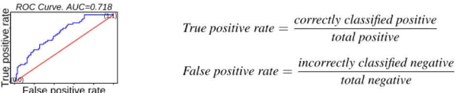
ROC Curve. AUC=0.718
True positive rate=correctly classified positive total positive
False positive rate= incorrectly classified negative total negative
Figure 1:An example of ROC curve. The line connecting(0,0)and(1,1), corresponding to random classification, is drawn for reference. The true positive (negative) rate is sometimes referred to as the sensitivity (resp. specificity) in this context.
In the following sections, we give a detailed statistical analysis of the relationship between the AUC and the error rate, including the first exact expression of the expected value and the variance of the AUC for a fixed error rate.2 We show that, under certain conditions, the global function optimized by the RankBoost algorithm is exactly the AUC. We report the results of our experiments with RankBoost in several datasets and demonstrate the benefits of an algorithm specifically designed to globally optimize the AUC over other existing algorithms optimizing an approximation of the AUC or only locally optimizing the AUC.
2
Definition and properties of the AUC
The Receiver Operating Characteristics (ROC) curves were originally developed in signal detection theory [3] in connection with radio signals, and have been used since then in many other applications, in particular for medical decision-making. Over the last few years, they have found increased interest in the machine learning and data mining communities for model evaluation and selection [12, 10, 4, 9, 15, 2].
The ROC curve for a binary classification problem plots the true positive rate as a function of the false positive rate. The points of the curve are obtained by sweeping the classifica-tion threshold from the most positive classificaclassifica-tion value to the most negative. For a fully random classification, the ROC curve is a straight line connecting the origin to(1,1). Any improvement over random classification results in an ROC curve at least partially above this straight line. Fig. (1) shows an example of ROC curve. The AUC is defined as the area under the ROC curve and is closely related to the ranking quality of the classification as shown more formally by Lemma 1 below.
Consider a binary classification task withmpositive examples andnnegative examples. We will assume that a classifier outputs a strictly ordered list for these examples and will denote by1Xthe indicator function of a setX.
Lemma 1 ([8]) Letcbe a fixed classifier. Letx1, . . . , xmbe the output ofcon the positive
examples andy1, . . . , ynits output on the negative examples. Then, the AUC, A, associated
tocis given by: A= Pm i=1 Pn j=11xi>yj mn (1)
that is the value of the Wilcoxon-Mann-Whitney statistic [8].
Proof. The proof is based on the observation that the AUC value is exactly the probability P(X > Y)whereX is the random variable corresponding to the distribution of the out-puts for the positive examples andY the one corresponding to the negative examples [7]. The Wilcoxon-Mann-Whitney statistic is clearly the expression of that probability in the discrete case, which proves the lemma [8].
Thus, the AUC can be viewed as a measure based on pairwise comparisons between classi-fications of the two classes. With a perfect ranking, all positive examples are ranked higher than the negative ones andA= 1. Any deviation from this ranking decreases the AUC.
2An attempt in that direction was made by [15], but, unfortunately, the authors’ analysis and the
m − (k − x) Positive examples θ Threshold x Negative examples k − x Positive examples n − x Negative examples
Figure 2:For a fixed number of errorsk, there may bex,0≤x≤k, false negative examples.
3
The Expected Value of the AUC
In this section, we compute exactly the expected value of the AUC over all classifications with a fixed number of errors and compare that to the error rate.
Different classifiers may have the same error rate but different AUC values. Indeed, for a given classification thresholdθ, an arbitrary reordering of the examples with outputs more thanθ clearly does not affect the error rate but leads to different AUC values. Similarly, one may reorder the examples with output less thanθwithout changing the error rate. Assume that the number of errorskis fixed. We wish to compute the average value of the AUC over all classifications withkerrors. Our model is based on the simple assumption that all classifications or rankings withkerrors are equiprobable. One could perhaps argue that errors are not necessarily evenly distributed, e.g., examples with very high or very low ranks are less likely to be errors, but we cannot justify such biases in general.
For a given classification, there may bex,0 ≤x≤k, false positive examples. Since the number of errors is fixed, there arek−xfalse negative examples. Figure 3 shows the cor-responding configuration. The two regions of examples with classification outputs above and below the threshold are separated by a vertical line. For a givenx, the computation of the AUC,A, as given by Eq. (1) can be divided into the following three parts:
A= A1+A2+A3
mn , with (2) A1= the sum over all pairs(xi, yj)withxiandyjin distinct regions;
A2= the sum over all pairs(xi, yj)withxiandyjin the region above the threshold;
A3= the sum over all pairs(xi, yj)withxiandyjin the region below the threshold.
The first term,A1, is easy to compute. Since there are(m−(k−x))positive examples
above the threshold andn−xnegative examples below the threshold,A1is given by:
A1= (m−(k−x))(n−x) (3)
To computeA2, we can assign to each negative example above the threshold a position
based on its classification rank. Let position one be the first position above the threshold and letα1< . . . < αxdenote the positions in increasing order of thexnegative examples
in the region above the threshold. The total number of examples classified as positive is N =m−(k−x) +x. Thus, by definition ofA2, A2= x X i=1 (N−αi)−(x−i) (4)
where the first termN−αirepresents the number of examples ranked higher than theith
example and the second termx−idiscounts the number of negative examples incorrectly ranked higher than theith example. Similarly, letα0
1< . . . < α0k−xdenote the positions of
thek−xpositive examples below the threshold, counting positions in reverse by starting from the threshold. Then,A3is given by:
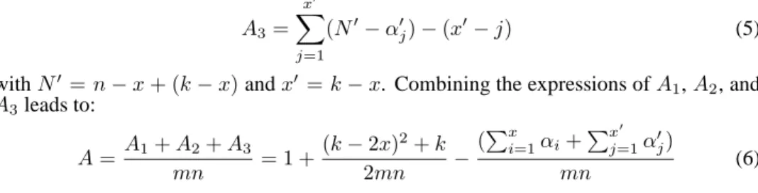
A3= x0 X j=1 (N0−α0 j)−(x 0−j) (5)
withN0 =n−x+ (k−x)andx0 =k−x. Combining the expressions ofA
1,A2, and A3leads to: A=A1+A2+A3 mn = 1 + (k−2x)2+k 2mn − (Pxi=1αi+Px 0 j=1α 0 j) mn (6)
Lemma 2 For a fixedx, the average value of the AUCAis given by: < A >x= 1− x n+ k−x m 2 (7)
Proof. The proof is based on the computation of the average values ofPxi=1αi and
Px0
j=1α
0
j for a givenx. We start by computing the average value< αi >xfor a given
i,1≤i≤x. Consider all the possible positions forα1. . . αi−1andαi+1. . . αx, when the
value ofαiis fixed at sayαi =l. We havei≤l ≤N−(x−i)since there need to be at
leasti−1positions beforeαiandN−(x−i)above. There arel−1possible positions for
α1. . . αi−1andN −lpossible positions forαi+1. . . αx. Since the total number of ways
of choosing thexpositions forα1. . . αxout ofN is Nx, the average value< αi>xis:
< αi>x= PN−(x−i) l=i l l−1 i−1 N−l x−i N x (8) Thus, < x X i=1 αi>x= Px i=1 PN−(x−i) l=i l l−1 i−1 N−l x−i N x = PN l=1l Px i=1 l−1 i−1 N−l x−i N x (9)
Using the classical identity:P p1+p2=p u p1 v p2 = u+vp , we can write: < x X i=1 αi>x= PN l=1l N−1 x−1 N x = N(N+ 1) 2 N−1 x−1 N x = x(N+ 1) 2 (10) Similarly, we have: < x0 X j=1 α0 j >x= x0(N0+ 1) 2 (11)
Replacing< Pxi=1αi >x and<
Px0
j=1α0j >x in Eq. (6) by the expressions given by
Eq. (10) and Eq. (11) leads to: < A >x= 1 + (k−2x)2+k−x(N+ 1)−x0(N0+ 1) 2mn = 1− x n+ k−x m 2 (12)
which ends the proof of the lemma.
Note that Eq. (7) shows that the average AUC value for a givenxis simply one minus the average of the accuracy rates for the positive and negative classes.
Proposition 1 Assume that a binary classification task with mpositive examples andn
negative examples is given. Then, the expected value of the AUCAover all classifications withkerrors is given by:
< A >= 1− k m+n− (n−m)2(m+n+ 1) 4mn k m+n− Pk−1 x=0 m+n x Pk x=0 m+n+1 x ! (13)
Proof. Lemma 2 gives the average value of the AUC for a fixed value ofx. To compute the average over all possible values ofx, we need to weight the expression of Eq. (7) with the total number of possible classifications for a givenx. There are N
x
possible ways of choosing the positions of thexmisclassified negative examples, and similarly Nx00
possible ways of choosing the positions of thex0=k−xmisclassified positive examples. Thus, in view of Lemma 2, the average AUC is given by:
< A >= Pk x=0 N x N0 x0 (1− nx+ k−x m 2 ) Pk x=0 N x N0 x0 (14)
0.0 0.1 0.2 0.3 0.4 0.5 0.5 0.6 0.7 0.8 0.9 1.0 Error rate Mean value of the AUC
r=0.01 r=0.05 r=0.1 r=0.25 r=0.5 0.0 0.1 0.2 0.3 0.4 0.5 .00 .05 .10 .15 .20 .25 Error rate Relative standard deviation r=0.01
r=0.05 r=0.1
r=0.25
r=0.5
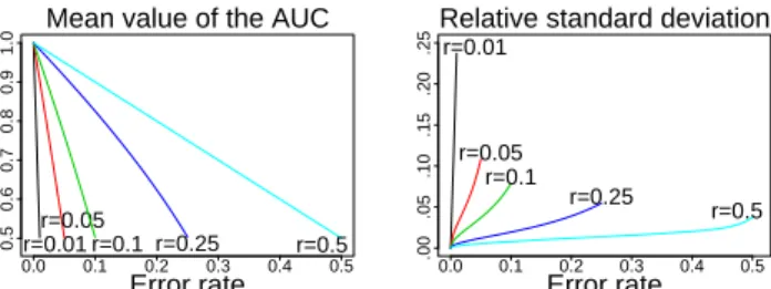
Figure 3:Mean (left) and relative standard deviation (right) of the AUC as a function of the error rate. Each curve corresponds to a fixed ratio ofr=n/(n+m). The average AUC value monotonically increases with the accuracy. Forn = m, as for the top curve in the left plot, the average AUC coincides with the accuracy. The standard deviation decreases with the accuracy, and the lowest curve corresponds ton=m.
This expression can be simplified into Eq. (13)3using the following novel identities:
k X x=0 N x ! N0 x0 ! = k X x=0 n+m+ 1 x ! (15) k X x=0 x N x ! N0 x0 ! = k X x=0 (k−x)(m−n) +k 2 n+m+ 1 x ! (16) that we obtained by using Zeilberger’s algorithm4and numerous combinatorial ’tricks’. From the expression of Eq. (13), it is clear that the average AUC value is identical to the accuracy of the classifier only for even distributions (n=m). Forn6= m, the expected value of the AUC is a monotonic function of the accuracy, see Fig. (3)(left). For a fixed ratio ofn/(n+m), the curves are obtained by increasing the accuracy fromn/(n+m)
to1. The average AUC varies monotonically in the range of accuracy between0.5and
1.0. In other words, on average, there seems nothing to be gained in designing specific learning algorithms for maximizing the AUC: a classification algorithm minimizing the error rate also optimizes the AUC. However, this only holds for the average AUC. Indeed, we will show in the next section that the variance of the AUC value is not null for any ratio n/(n+m)whenk6= 0.
4
The Variance of the AUC
LetD = mn+(k−2x)22+k,a = Pxi=1αi,a0 =
Px0
j=1α0j, andα = a+a0. Then, by
Eq. (6),mnA=D−α. Thus, the variance of the AUC,σ2(A), is given by:
(mn)2σ2(A) = <(D−α)2−(< D >−< α >)2> (17) = < D2 >−< D >2 +< α2 >−< α >2 −2(< αD >−< α >< D >) As before, to compute the average of a termX over all classifications, we can first deter-mine its average< X >xfor a fixedx, and then use the functionF defined by:
F(Y) = Pk x=0 N x N0 x0 Y Pk x=0 N x N0 x0 (18)
and< X >=F(< X >x). A crucial step in computing the exact value of the variance of
the AUC is to determine the value of the terms of the type< a2>
x=<(Pxi=1αi)2>x.
3
An essential difference between Eq. (14) and the expression given by [15] is the weighting by the number of configurations. The authors’ analysis leads them to the conclusion that the average AUC is identical to the accuracy for all ratiosn/(n+m), which is false.
4
Lemma 3 For a fixedx, the average of(Pxi=1αi)2is given by: < a2>x= x(N + 1) 12 (3N x+ 2x+N) (19) Proof. By definition ofa,< a2> x=b+ 2cwith: b=< x X i=1 α2i >x c=< x X 1≤i<j≤x αiαj>x (20)
Reasoning as in the proof of Lemma 2, we can obtain: b= Px i=1 PN−(x−i) l=i l2 l−1 i−1 N−l x−i N x = N X l=1 l2 N−1 x−1 N x = (N+ 1)(2N+ 1)x 6 (21)
To computec, we start by computing the average value of< αiαj >x, for a given pair(i, j)
withi < j. As in the proof of Lemma 2, consider all the possible positions ofα1. . . αi−1,
αi+1. . . αj−1, andαj+1. . . αx whenαi is fixed atαi = l, andαj is fixed atαj = l0.
There arel−1 possible positions for the α1. . . αi−1, l0−l −1 possible positions for
αi+1. . . αj−1, andN−l0possible positions forαj+1. . . αx. Thus, we have:
< αiαj >x= P i≤l<l0≤N−(x−j)ll0 l−1 i−1 l0−l−1 j−i−1 N−l0 x−j N x (22) and c= P l<l0ll 0P m1+m2+m3=x−2 l−1 m1 l0−l−1 m2 N−l0 m3 N x (23)
Using the identityP
m1+m2+m3=x−2 l−1 m1 l0−l−1 m2 N−l0 m3 = Nx−−22 , we obtain: c=(N+ 1)(3N+ 2)x(x−1) 24 (24)
Combining Eq. (21) and Eq. (24) leads to Eq. (19).
Proposition 2 Assume that a binary classification task with mpositive examples andn
negative examples is given. Then, the variance of the AUCAover all classifications with
kerrors is given by:
σ2(A) = F((1− x n+ k−x m 2 ) 2)−F((1− x n+ k−x m 2 )) 2+ (25) F(mx 2+n(k−x)2+ (m(m+ 1)x+n(n+ 1)(k−x))−2x(k−x)(m+n+ 1) 12m2n2 )
Proof. Eq. (18) can be developed and expressed in terms ofF,D,a, anda0:
(mn)2σ2(A) =F([D−< a+a0> x]2)−F(D−< a+a0 >x)2+ F(< a2> x−< a >2x) +F(< a 02> x−< a0>2x) (26)
The expressions for< a >x and < a0 >x were given in the proof of Lemma 2, and
that of < a2 >
x by Lemma 3. The following formula can be obtained in a similar
way:< a02>
x=x
0(N0+1)
12 (3N
0x0+ 2x0+N0). Replacing these expressions in Eq. (26) and further simplifications give exactly Eq. (25) and prove the proposition.
The expression of the variance is illustrated by Fig. (3)(right) which shows the value of one standard deviation of the AUC divided by the corresponding mean value of the AUC. This figure is parallel to the one showing the mean of the AUC (Fig. (3)(left)). Each line is obtained by fixing the ration/(n+m)and varying the number of errors from 1 to the size of the smallest class. The more uneven class distributions have the highest variance, the variance increases with the number of errors. These observations contradict the inexact claim of [15] that the variance is zero for all error rates with even distributionsn=m. In Fig. (3)(right), the even distributionn=mcorresponds to the lowest dashed line.
Dataset Size # of n
n+m AUCsplit[4] RankBoost
Attr. (%) Accuracy (%) AUC (%) Accuracy (%) AUC (%) Breast-Wpbc 194 33 23.7 69.5±10.6 59.3±16.2 65.5±13.8 80.4±8.0 Credit 653 15 45.3 81.0±7.4 94.5±2.9 Ionosphere 351 34 35.9 89.6±5.0 89.7±6.7 83.6±10.9 98.0±3.3 Pima 768 8 34.9 72.5±5.1 76.7±6.0 69.7±7.6 84.8±6.5 SPECTF 269 43 20.4 67.3 93.4 Page-blocks 5473 10 10.2 96.8±0.2 95.1±6.9 92.0±2.5 98.5±1.5 Yeast (CYT) 1484 8 31.2 71.1±3.6 73.3±4.0 45.3±3.8 78.5±3.0
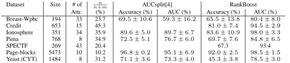
Table 1: Accuracy and AUC values for several datasets from the UC Irvine repository. The values for RankBoost are obtained by 10-fold cross-validation. The values for AUCsplit are from [4].
5
Experimental Results
Proposition 2 above demonstrates that, for uneven distributions, classifiers with the same fixed (low) accuracy exhibit noticeably different AUC values. This motivates the use of algorithms directly optimizing the AUC rather than doing so indirectly via minimizing the error rate. Under certain conditions, RankBoost [5] can be viewed exactly as an algorithm optimizing the AUC. In this section, we make the connection between RankBoost and AUC optimization, and compare the performance of RankBoost to two recent algorithms proposed for optimizing an approximation [15] or locally optimizing the AUC [4]. The objective of RankBoost is to produce a ranking that minimizes the number of incor-rectly ordered pairs of examples, possibly with different costs assigned to the mis-rankings. When the examples to be ranked are simply two disjoint sets, the objective function mini-mized by RankBoost is rloss= m X i=1 n X j=1 1 m 1 n1xi≤yj (27)
which is exactly one minus the Wilcoxon-Mann-Whitney statistic. Thus, by Lemma 1, the objective function maximized by RankBoost coincides with the AUC.
RankBoost’s optimization is based on combining a number of weak rankings. For our experiments, we chose as weak rankings threshold rankers with the range{0,1}, similar to the boosted stumps often used by AdaBoost [6]. We used the so-called Third Method of RankBoost for selecting the best weak ranker. According to this method, at each step, the weak threshold ranker is selected so as to maximize the AUC of the weighted distribution. Thus, with this method, the global objective of obtaining the best AUC is obtained by selecting the weak ranking with the best AUC at each step.
Furthermore, the RankBoost algorithm maintains a perfect 50-50% distribution of the weights on the positive and negative examples. By Proposition 1, for even distributions, the mean of the AUC is identical to the classification accuracy. For threshold rankers like step functions, or stumps, there is no variance of the AUC, so the mean of the AUC is equal to the observed AUC. That is, instead of viewing RankBoost as selecting the weak ranker with the best weighted AUC value, one can view it as selecting the weak ranker with the lowest weighted error rate. This is similar to the choice of the best weak learner for boosted stumps in AdaBoost. So, for stumps, AdaBoost and RankBoost differ only in the updat-ing scheme of the weights: RankBoost updates the positive examples differently from the negative ones, while AdaBoost uses one common scheme for the two groups.
Our experimental results corroborate the observation that RankBoost is an algorithm op-timizing the AUC. RankBoost based on boosted stumps obtains AUC values that are sub-stantially better than those reported in the literature for algorithms designed to locally or approximately optimize the AUC. Table 1 compares the results of RankBoost on a number of datasets from the UC Irvine repository to the results reported by [4]. The results for RankBoost are obtained by 10-fold cross-validation. For RankBoost, the accuracy and the best AUC values reported on each line of the table correspond to the same boosting step. RankBoost consistently outperforms AUCsplit in a comparison based on AUC values, even for the datasets such as Breast-Wpbc and Pima where the two algorithms obtain similar ac-curacies. The table also lists results for the UC Irvine Credit Approval and SPECTF heart dataset, for which the authors of [15] report results corresponding to their AUC optimiza-tion algorithms. The AUC values reported by [15] are no better than92.5%for the Credit
Approval dataset and only87.5%for the SPECTF dataset, which is substantially lower. From the table, it is also clear that RankBoost is not an error rate minimization algorithm. The accuracy for the Yeast (CYT) dataset is as low as45%.
6
Conclusion
A statistical analysis of the relationship between the AUC value and the error rate was given, including the first exact expression of the expected value and standard deviation of the AUC for a fixed error rate. The results offer a better understanding of the effect on the AUC value of algorithms designed for error rate minimization. For uneven distributions and relatively high error rates, the standard deviation of the AUC suggests that algorithms designed to optimize the AUC value may lead to substantially better AUC values. Our experimental results using RankBoost corroborate this claim.
In separate experiments we have observed that AdaBoost achieves significantly better er-ror rates than RankBoost (as expected) but that it also leads to AUC values close to those achieved by RankBoost. It is a topic for further study to explain and understand this prop-erty of AdaBoost. A partial explanation could be that, just like RankBoost, AdaBoost maintains at each boosting round an equal distribution of the weights for positive and neg-ative examples.
References
[1] L. Breiman, J. H. Friedman, R. A. Olshen, and C. J. Stone. Classification and
Regres-sion Trees. Wadsworth International, Belmont, CA, 1984.
[2] J-H. Chauchat, R. Rakotomalala, M. Carloz, and C. Pelletier. Targeting customer groups using gain and cost matrix; a marketing application. Technical report, ERIC Laboratory - University of Lyon 2, 2001.
[3] J. P. Egan. Signal Detection Theory and ROC Analysis. Academic Press, 1975. [4] C. Ferri, P. Flach, and J. Hern´andez-Orallo. Learning decision trees using the area
under the ROC curve. In ICML-2002. Morgan Kaufmann, 2002.
[5] Y. Freund, R. Iyer, R. E. Schapire, and Y. Singer. An efficient boosting algorithm for combining preferences. In ICML-98. Morgan Kaufmann, San Francisco, US, 1998. [6] Yoav Freund and Robert E. Schapire. A decision theoretical generalization of
on-line learning and an application to boosting. In Proceedings of the Second European
Conference on Computational Learning Theory, volume 2, 1995.
[7] D. M. Green and J. A Swets. Signal detection theory and psychophysics. New York: Wiley, 1966.
[8] J. A. Hanley and B. J. McNeil. The meaning and use of the area under a receiver operating characteristic (ROC) curve. Radiology, 1982.
[9] M. C. Mozer, R. Dodier, M. D. Colagrosso, C. Guerra-Salcedo, and R. Wolniewicz. Prodding the ROC curve. In NIPS-2002. MIT Press, 2002.
[10] C. Perlich, F. Provost, and J. Simonoff. Tree induction vs. logistic regression: A learning curve analysis. Journal of Machine Learning Research, 2003.
[11] G. Piatetsky-Shapiro and S. Steingold. Measuring lift quality in database marketing. In SIGKDD Explorations. ACM SIGKDD, 2000.
[12] F. Provost and T. Fawcett. Analysis and visualization of classifier performance: Com-parison under imprecise class and cost distribution. In KDD-97. AAAI, 1997. [13] S. Rosset. Ranking-methods for flexible evaluation and efficient comparison of
2-class models. Master’s thesis, Tel-Aviv University, 1999.
[14] S. Rosset, E. Neumann, U. Eick, N. Vatnik, and I. Idan. Evaluation of prediction models for marketing campaigns. In KDD-2001. ACM Press, 2001.
[15] L. Yan, R. Dodier, M. C. Mozer, and R. Wolniewicz. Optimizing Classifier Perfor-mance Via the Wilcoxon-Mann-Whitney Statistics. In ICML-2003, 2003.