A method for under-sampled ecological network data analysis: plant-pollination as case study

129

A

METHOD FOR UNDER

-

SAMPLED ECOLOGICAL NETWORK DATA

ANALYSIS

:

PLANT

-

POLLINATION AS CASE STUDY

Peter B. Sørensen

1,

_{*, Christian F. Damgaard}

1

_{, Beate Strandberg}

1

_{, Yoko L. Dupont}

2

_{, Marianne B.}

Pedersen

1

_{, Luisa G. Carvalheiro}

3,4

_{, Jacobus C. Biesmeijer}

4

_{, Jens Mogens Olsen}

2

_{, Melanie Hagen}

2

_{, Simon}

G. Potts

5

1_{Aarhus University, Bioscience, Vejlsøvej 25, P.O.Box 314, 8600 Silkeborg, Denmark} 2_{Aarhus University, Bioscience, NyMunkegade 114, 8000 Aarhus C, Denmark}

3_{Institute of Integrative and Comparative Biology, University of Leeds, Leeds LS2 9JT, UK} 4 _{NCB-Naturalis, postbus 9517, 2300 RA, Leiden, The Netherlands}

5_{University of Reading, School of Agriculture, Policy and Development, UK}

AbstractIn this paper, we develop a method, termed the Interaction Distribution (ID) method, for analysis of

quantitative ecological network data. In many cases, quantitative network data sets are under-sampled, i.e. many interactions are poorly sampled or remain unobserved. Hence, the output of statistical analyses may fail to differentiate between patterns that are statistical artefacts and those which are real characteristics of ecological networks. The ID method can support assessment and inference of under-sampled ecological network data. In the current paper, we illustrate and discuss the ID method based on the properties of plant-animal pollination data sets of flower visitation frequencies. However, the ID method may be applied to other types of ecological networks. The method can supplement existing network analyses based on two definitions of the underlying probabilities for each combination of pollinator and plant species: (1), pi,j: the probability for a visit made by the i’th pollinator species to take place on the j’th plant species; (2), qi,j: the probability for a visit received by the j’th plant species to be made by the i’th pollinator. The method applies the Dirichlet distribution to estimate these two probabilities, based on a given empirical data set. The estimated mean values for pi,j and qi,j reflect the relative differences between recorded numbers of visits for different pollinator and plant species, and the estimated uncertainty of pi,j and qi,j decreases with higher numbers of recorded visits.

Keywords: Ecological network, Bayesian method, plant-animal pollination data analysis, under-sampled data sets

I

NTRODUCTION

Plant-pollinator interactions are important for maintenance of biological diversity, and pollination is a valuable ecosystem function for both wild plant communities and agricultural production (Potts et al. 2010). Hence, anthropogenic changes to the environment have negative effects on plants and pollinators, and hence pollination is seen as an ecological network (e.g. Biesmeijer et al. 2006; Hegland et al. 2009). To better understand mechanisms behind such consequences, modelling, interpretation and handling of pollination data as ecological networks are necessary steps (Potts et al., 2011).

During the past decade, ecologists have become increasingly interested in ecological networks, and network analysis is applied to complex patterns of interactions among species in food webs, mutualistic and host-parasite networks (reviewed by Ings et al. 2009). The application of methods of the network analysis has gained new insights into their topological patterns, e.g. degree distributions (Jordano et al. 2003; Vazquez 2005), nestedness (Bascompte et al. 2003;

Dupont et al. 2003), modularity (Olesen et al. 2007), small world properties (Olesen et al. 2006), patterns of generalization/specialization (i.e. level of degree) ( Bascompte et al. 2006; Olesen and Jordano 2002; Vazquez and Aizen 2003), tolerance to species extinction (Fortuna and Bascompte 2006; Memmott et al. 2004), and phenological shifts (Kaiser-Bunbury et al. 2010; Memmott et al. 2007). Network data are often qualitative, i.e. include only presence/absence information about species and links; however, quantitative networks, which include link strength, i.e. visitor/visitation frequencies, are becoming increasingly available, and network descriptors based on quantitative data have been developed (e.g. Bersier et al. 2002). Such network descriptors as well as the outcome of studies on ecological networks (e.g. extinction simulations) are highly susceptible to the overall number of interactions detected (e.g. stability; see Banasek-Richer et al. 2009; Dormann et al. 2009).

The validity of an interpretation derived from a description using network theory depends on the properties of the underlying empirical data, and the different sampling methods used in pollination network field studies have different constraints that deviate from randomness (e.g. Gibson et al. 2011). Gathering pollination network data sets is resource and time consuming and they are nearly always Received 8 August 2011, accepted 12 December 2011

under-sampled because species or interactions easily escape observation (Olesen et al. 2010; Vazquez et al. 2009). Moreover, pollination networks are temporally highly dynamic, i.e. species and interactions are continuously changing (Alarcón et al. 2008; ; Dupont et al. 2009; Olesen et al. 2008; Petanidou et al. 2008). In most empirical studies, data collection is plant focused (Olesen et al. 2010), i.e. a fixed number of plant species are observed for visiting pollinators. This may impede our understanding of network organization and function. In particular, interactions may remain undetected because most flower visits are rare, of short duration, and usually do not leave traces on the flower. Thus, the number of recorded visits is only a small subset of the actual visits made by a species (Blüthgen et al. 2010; Goldwasser and Roughgarden 1997). Obviously, the problem of under sampling is most severe for larger networks. As a rule of thumb, the sampling effort has to increase in proportion to the number of interactions, i.e. combinations of a pollinator species and a plant species.

The following question is addressed in this paper in order to facilitate further progress for application of network data:

How can we improve the applicability of data sets to support network analysis without misinterpretation due to sampling bias and inadequate number of data records?

The problem of under sampling has been statistically investigated and modelled (Dormann et al. 2009; Vazquez and Aizen 2003) and assuming random sampling. In this paper, we propose and discuss a Bayesian approach called the ID method and a general concept model to link experiment and data analysis to see how this can supplement existing methods and, thereby, contribute to better applicability. Thus, the hypothesis of this paper is:

A Bayesian approach and a conceptual model can improve the applicability of data sets by setting up a description of the probability for a record to involve a specific combination of a visitor (pollinator species) and a receptor (plant species)!

This paper will describe the suggested methods and discuss the outcome under on the following headlines:

- How can the conceptual model clarify the governing assumptions underpinning all application of under-sampled data sets in any type of network analysis?

- What are the governing assumptions underpinning the ID method compared to the alternatives?

- How can the ID method increase the understanding in network analysis?

- How easy is the application of the ID method?

- The method is described in the next paragraph followed by the discussion to address the questions above.

M

ETHODS

Two definitions of underlying probabilities of visits are applied for each visit:

- pi,j: the pollinator focused probability. Out of all visits by the i’th pollinator species, pi,j is the probability of a visit

to take place in the j’th plant species. This is a measure of a pollinator species preference for a plant species.

- qi,j: the plant focused probability. Out of all visits done in the j’th plant species, qi,j is the probability of a visit to be done by the i’th pollinator. This is a measure of pollinator species i’s preference for visiting plant species

j, relative to the preference of other pollinator species to visit the same plant species.

Thus, the visits to each plant species is considered as a multinomial process, where the individual pollinator “decides” to visit a plant species with some unknown probability. The task of this paper is to estimate possible intervals for this probability based on empirical data.

Conceptual model

The conceptual model is described based on sets, where the set containing all single visits between a single pollinator and plant species that took place in the area and period of study is denoted A. Every single visit is an element in the set

A. Set A is divided into subsets as Apolli and Aplj, where

Apolli is the subset of A, containing all elements in A where pollinator i performs the visits and Aplj is a subset of A, containing all elements in A where the plant j is being visited. All visits will involve one and only one pollinator species (i) and plant species (j), respectively, and thus are single elements that belong to both the subsets Apolli and Aplj. A subset of A is defined as the set containing all recorded

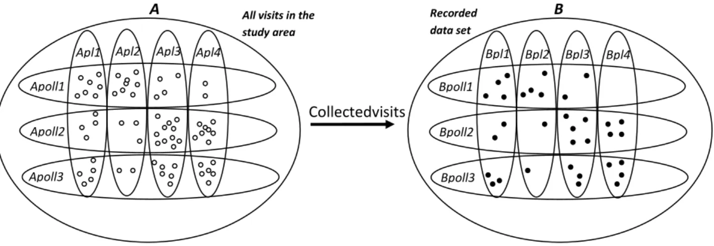
(collected) visits and denoted as set B, and for set B the subsets Bpolli and Bplj are defined for respective pollinator and plant species. The conceptual model is illustrated in Fig. 1 for three pollinator species and four plant species. Hence, if a visit is recorded in the data set, then the visit is an element that belongs to both set A, Apolli and Aplj and set B,

Bpolli and Bplj, respectively.

If all visits in set B are random observations from A

without bias for any pollinator or plant species, then B is claimed to be randomly collected. Thus, a random collection assumes that the data collector is not more likely to record visits by some species of pollinators, e.g. large conspicuous bumble bees, than others, e.g. small flies. A fully random collection also assumes that the plant species are randomly selected. Thus, if plant species Pl1 receives twice as many visits as plant species Pl2, then the probability of an observer, in a fully random collection, to observe a visit by pollinator of Pl1 is twice as high as the probability of observing a pollinator visiting Pl2.

Thus, for the “ideal” random observer, every visit in the study area is equally likely to be observed, and set B is a random selection of some of the elements in set A. However, for empirical data sets, the set B is rarely a random subset of

A and its applicability for analysis is, thus, constrained or to some degree uncertain. Two typical cases of “non-randomness” or bias can be defined in the following way:

Pollinator focused sampling, has random sampling within Bpolli, but not between different pollinators and, thus, only allows estimating pi,j. This can be illustrated in Fig. 1 as a situation where an element placed in Apoll1 is

Figure 1. Illustration of the concept model, including three pollinator species and four plant species, with the set of all interactions between pollinator and plant species (A) and a subset of recorded interactions (B). The definition of sets in the model concept follows the definitions in the text, where every single dot ( ) represents is a visit.

more likely to be collected than an element placed in Apoll2, but within Apoll1 the likelihood for an element to be collected is the same for all plant species (Apl1-4). This type of randomness will be denoted ‘pollinator focused sampling’ and can be used only to estimate pi,j. Data generated with a pollinator focus, e.g. by tracking pollinator individuals visiting flowers, could be considered as pollinator focused sampling. Another reason behind this type of non-randomness (bias) could be that the observer has more focus on the large conspicuous bumble bees than on small flies. If this type of sampling is applied for generating data to feed network models, then a high connectivity for one pollinator species compared to others can be an artefact due to an extra intensive sampling effort for that specific pollinator species.

Plant focused sampling has random sampling within Bplj, but not between different plant species and, thus only allows estimating qi,j. This can be shown in Fig. 1 as a situation where an element in Apl1 is more likely to be collected than an element in Apl2, but within Apl1 the likelihood of a collection from one of the pollinator species (Apoll1-4) is the same. A sampling method that will mimic this situation is an approach, where the plant species are recorded by an observer who is waiting for the pollinators to arrive to the focused upon plant individual. If this type of sampling is applied for generating data to feed network models, then a high connectivity for one plant species compared to other plants in the data set can be an artefact due to an extra intensive sampling effort for that specific plant species.

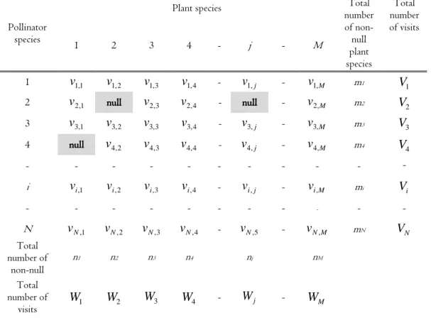
The data set B is used to make a data table (Table 1) by summing the number of elements for every combination of pollinator and plant species. This table is termed an interaction frequency matrix. Row i in Table 1 contains all visits by Bpolli and column j contains all visits received by

Bplj. The value vi,jis, thus, the number of visits, equivalent to the number of elements in Bpolli∩Bplj.

Modelequations

Number of total recorded visits by the i’th pollinator species on any plant species in the data set is

∑

=

= M

1 j

ij

i v

V 1a

Number of total recorded visits to plant species j by any pollinator species is

∑

= = N 1 i

ij

j v

W 1b

Eqs. 1a and b are based on the definitions in Table 1. A row of vi,1,vi,2,...,vi,M values in Table 1 can be considered as a vector vj. The number shows that the pollinator i has visited the plant j a total of vvvvi,ji,ji,ji,j times. When pollinator i makes a visit, then the probability for this visit to take place in plant j is pi,j If it is a priori known that pollinator species i will never visit plant species j, then this combination of i and j is denoted “null” in Table 1, and vvvvi,ji,ji,ji,j must necessarily have been recorded as zero in the data set. This situation will occur if plant and pollinator species mismatch e.g. in phenology or morphology or in season (Olesen et al. 2010). It follows that the probability for a pollinator species to visit the plant species must be zero for all “null” combinations of i and j, thus, vi,j ≡ 0 for all combinations of i and j values having a “null” for vi,j. On the other hand, a value of vi,j=0 will not necessarily be a “null”

value, as it could imply that the pollinator species i so seldom visiting plant j that such a visit is not recorded in the data set or it may be an unknown null value.

In conclusion, if the pi,j values are known, it will be possible to set up a statistical multinomial model to predict the distributions of possible numbers of visits made by a pollinator species to different plant species in a data set. The challenge is that the pi,j values are unknown and, hence, should be estimated from an empirical data set (Table 1). The Dirichlet distribution can estimate the distribution of possible pi,j values for the multinomial distribution based on empirical data (Frigyik et al. 2010).Thus, it follows that if we have the correct values for pi,j, then we can estimate the distribution of possible vi,j values, using a multinomial distribution as a statistical model based on the total number All visits in the

study area

Bpl2 Bpoll1

Bpoll2

Bpoll3

Bpl1 Bpl3 Bpl4

Collectedvisits

A

B

Apoll1

Apoll2

Apoll3

Apl1 Apl2 Apl3 Apl4

Recorded data set

Pollinator species

Plant species Total

number of non-null plant species Total number of visits

1 2 3 4 - j - M

1

v

1,1

v

1,2

v

1,3

v

1,4 -

v

1,j -

v

1,M m1

V

1

2

v

2,1 nullnullnullnull

v

2,3

v

2,4 - nullnullnullnull -

v

2,M m2

V

₂

3

v

3,1

v

3,2

v

3,3

v

3,4 -

v

3,j -

v

3,M m3

V

3

4 nullnullnullnull

v

_4,2

v

_4,3

v

_4,4 -

v

_4,j -

v

_4,M m4

4

V

- - - -

i

v

i,1

v

i,2

v

i,3

v

i,4 -

v

i,j -

v

i,M mi

V

i

- - - -

N

v

N,1

v

N,2

v

N,3

v

N,4 -

v

N,5 -

v

N,M mN

V

N Total

number of non-null

n1 n2 n3 n4 nj nM

Total number of

visits 1

W

W

₂

W

3

W

4 -

W

j -

W

M

of observations. However, because the pi,j values are unknown, we can use the data set to find possible values based on the assumption that a multinomial distribution is more likely to result in the observed data set for some pi,j values compared to others. In Bayesian terms, this means that the Dirichlet distribution can be used to find this distribution of pi,j values as the conjugate prior for the multinomial distribution (Frigyi et al. 2010). However, this paper will not go deeper into the background of Bayesian analysis and will, thus, take this statement for granted. For comprehensive data sets (high sampling effort), the Dirichlet distribution will be “narrow” and, thus, estimate the pi,j value as narrow (certain) intervals, while a sparse data set (low sampling effort) will result in a broad and more uncertain estimate of the pi,j values.

The Dirichlet distribution Dir (α) for pi, where pi is the vector of the probabilities pi,1,…pi,m , andα is theparameter vectorα1,…,αm is

(

)

∑

_{[ ]}

_{( )}

_∏

=

( )

− = = ⋅       = M 1 j 1 j i, M 1 j j M 1 j j i Vi j p , p f α α Γ α Γ α

C

2

Where and Γ

( )

is the gamma function (Evans et al. 2000). If there are no data (a priori) to consider,then the Dir (αι) is assumed to have unified distributions for all

pi,,1,…pi,m , which is equivalent to stating that “no data” is “no knowledge”. The Dirichlet distribution yields a unified distribution for pi,1,…pi,m when: α1,…,αm=1 and acts as conjugate prior for the multinomial distribution by

Dir(αi+vi)(Frigyik et al., 2010 ), where vi is the vector of

M i, i,2 i,1,v ,...,v

v (Countings in Table 1). Thus,

using α1,…,αm=1 for Dir(αi+vi),the distribution function becomes:

(

)

(

_[

₍

)

₎

_]

_∏

( )

∏

= = ⋅ + + = M 1 j v j i, M 1 j i,j

i i i i Vi j i, p 1 v m V v , p f Γ Γ 3

Both pi and vi are only defined for j values that are not “null” in the data set.

All the considerations above can be repeated for the probabilities qi,1,...qi,M and the vector vi of v1,j,v2,j,...,vN,jin order to investigate the probabilities for different pollinator species to visit plant species j. This yields a similar equation for qi,j ,

(

)

(

_[

₍

)

₎

_]

_∏

( )

∏

= = ⋅ + + = N 1 i v j i, M 1 j i,j

j j j j Wj j i, q 1 v n W v , q f Γ Γ 3b

Where qi is the vector of the probabilities qi,1,…qi,m. Both

qi and vi are only defined for i values that are not “null” in the data set.

The following necessary relations are true for the probabilities:

∑

= = M j j i

p

1

, 1 4a

The probability for a pollinator to visit any possible plant when it makes a visit is 1

Table 1. The data matrix of visitation data (interaction frequency matrix),with the recorded number of visits by pollinator i onto plant j. N and M are numbers of pollinator and plant species in the data set, respectively. The null values are used for combinations of pollinator species and plant species where visits are known to be impossible.

∑

= = N i j i q 1

, 1 4b

The probability of a plant receiving a visit from any possible pollinator when it gets a visit is 1

It can be shown (Frigyik et al., 2010) that the density distribution (marginal distributions) of pi,j and qi,j, respectively, can be described by the beta function as:

( )

p beta(1 v ;m V v 1)

fpij i,j = + i,j i + i − i,j − 5a

( )

i,j = (1+ i,j; i + i − i,j −1)

pij q beta v n W v

f 5b

The Beta distribution has some simple statistical properties (see e.g. Evans et al., 2000). Hence, using Eqs. 5a and b, we find mean (E) and variance (VAR) for pi,j and qi,j:

( )

i i j i j i

V

m

v

p

E

+ + = , , 1 6a

( )

i i j i j i

W

n

v

q

E

+ + = , , 1 6b

( ) ( )

(

( )

)

i i j i j i j i

V

m

p

E

p

E

p

VAR

+ + − ⋅ = 1 1 , , . 7a

( ) ( )

(

( )

)

j j j i j i j i W n q E q E q VAR + + − ⋅ = 1 1 , , . 7b

Increasing values for Vi and Wj will lead to a greater increase in the nominator relative to the denominator in Eqs. 7a and 7b, and VAR(), therefore, will decrease when the number of records is increased. Hence, pij and qi,j become increasingly precisely estimated for an increasing number of records. This also applies to cases where additional records are not related to specific pollinator or plant species (different i or j value).

It is possible to make a simplified uncertainty assessment of the under-sampled data sets based on the binominal distribution and pi,j or qi,j respectively.

) , , ( i,j i i,j

vij Binv V p

f = _8a

) , , ( i,j j i,j

vij Binv W q

f = _8b

Where j i i j

i V p

v

E( , )= ⋅ , _9a

j i j j

i W q

v

E( , )= ⋅ , 9b

If the values of pi,j and qi,j are assumed to be known or estimated using Eq. 6a or b, respectively, then it is possible to estimate the interval of “realistic” vi,j values that can be

recorded out of all Vi or Wj records for pollinator i. The variance of vi,j can be estimated in cases where the normal approximation is valid: Vi⋅pi,j >>1 or Wj⋅qi,j >>1and

(

1 ,

)

1

, ⋅ − >> ⋅ ij ij

i p p

V or Wj⋅qi,j⋅

(

1−qi,j

)

>>1 as )

1 ( )

(vi,j Vi pi,j pi,j

VAR ≈ ⋅ ⋅ − 10a

) 1 ( )

(vi,j Wj qi,j qi,j

VAR ≈ ⋅ ⋅ − 10b

Combining Eqs. 6a and b with 10a or 10b yields a simple rough estimate for the variance of vi,j:

      + + − ⋅ + + ≈ i i j i i i j i i j i V m v V m v V v

VAR , ,

, 1 1 ) 1 ( ) ( 11a         + + − ⋅ + + ≈ j j j i j i j i j j i W n v W n v W v

VAR , ,

, 1 1 ) 1 ( ) ( 11b

If the normal approximation is valid, then it will also be true that vi,j >>1and, in many cases, also

V

i >>

m

ior

j

j n

W >> , yielding the following simple but rough estimate for the variance:

      − ⋅ ≈ i j i j i j i V v v v VAR , ,

, ) 1

( 12a         − ⋅ ≈ j j i j i j i W v v v VAR , ,

, ) 1

( 12b

N

UMERICALEXAMPLEFORILLUSTRATION

The principle of the method is best illustrated by a simple artificial numerical example. Real data sets will, typically, be much larger, so a smaller numerical example is chosen for the purpose of illustration. The data set includes three pollinator species (rows) and two plant species (columns) (Table 2).

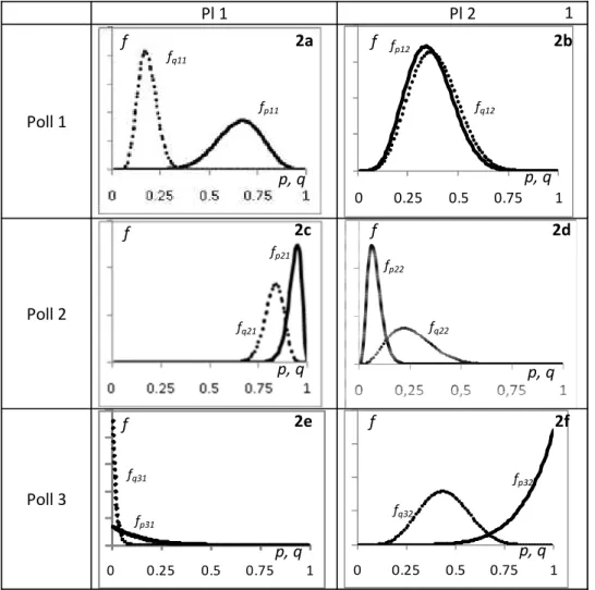
The distribution of p and q is calculated using Eqs. 5a and b, respectively, and the results are shown in Fig 2a-f.

The Poll 1 and Pl 1 combination in Table 2 shows a situation where Poll 1most frequently visits this plant and, thus, a density distribution (Fig. 2a) for p1,1 that is located mainly above 0.5. On the other hand, the plant species receives more visits from Poll 2, so the value of q1,1 is smaller Table 2. Illustrative data set for three pollinator and two plant species

Pl1 Pl2 Total

Poll1 10 5 15

Poll2 50 3 53

Poll3 0 6 6

1

Pl 1

Pl 2

Poll 1

0 0.25 0.5 0.75 1

Poll 2

Poll 3

0 0.25 0.5 0.75 1 0 0.25 0.5 0.75 1

fq11

fp11

fp12

fq12

fp22

fq22

fp21

fq21

fq31

fp31

fq32

fp32

f

f

f

f

f

f

p, q

p, q

p, q

p, q

p, q

p, q

2b

2a

2d

2c

2f

2e

than 0.5. The limited number of total recorded visits for Poll 1 results in a wider distribution (larger VAR()) of the

p1,1value compared to the stronger (smaller VAR()) determination of the q1,1 value. A similar relation, where the strength of the estimation is highly different, is also shown for the Poll 2 and Pl 2 combination (Fig. 2d), but the roles of pollinator and plant are reversed. The Poll 2 and Pl 1 combination (Fig. 2c) shows a situation with a larger number of records, yielding a good determination of both probabilities. Poll 3 only visited Pl 2 and was only recorded six times in total. From the data, one may conclude that Poll 3 is not visiting Pl 1. However, due to the low number of records, this may simply be a result of small sample size. The curve for p3,1 in Fig. 2e shows that the probability for Poll 3 to visit Pl 1, when Poll 3 is visiting either Pl 1 or 2, is less than 0.25, but markedly above zero. However, if the question is reversed, i.e. ’what is the probability of a visit to Pl 1 by Poll 3’ (q3,1), the result is dramatically different, i.e. a probability close to zero is highly probable due to a high number (60) of visits observed at Pl 1, but none were by Poll3, so in this case the ID method may have identified an unknown “null value”.

The Dirichlet distribution function (Eq. 3b) for Pl 2 is shown in Fig. 3.

The dynamics of the multivariate probability are shown in Fig 3. For instance, the distribution for q1,2 (visits by Poll

1 to Pl 2) depends on the value of q3,2, (visits of Poll 3 to Pl 2). Hence, if the q3,2 value is high, then it leaves smaller likelihood and variation for q1,2, because q3,2+q1,2+q2,2 = 1, which forces the density distribution for q1,2 to level out for larger values of q3,2.

The distribution functions listed in Fig. 2a-f indicate the sampling uncertainty for the data in Table 2, where a wide

Figure 3. The Dirichlet distribution function for Pl 2 showing q3,2 and q1,2, where q2,2 has been determined for all combinations of q3,2 and q1,2 as 1-q3,2-q1,2.

Figure 2a-f. Graphic display of eqs. 5 a and b for the data in Table 2, where the y-axis is the probability density for p and q, and the x-axis is the values of p and q (continuous line: function of p, dotted line: function of q).

distribution predicts a high uncertainty due to a limited number of records. However, it is also possible to make a simple assessment of the uncertainty based on Eqs. 11a or 12a if relatively many records (Vi⋅pi,j >>1 and

(

1 ,

)

1

, ⋅ − >> ⋅ ij ij

i p p

V ) are available. This can be

considered as a valid approximation for e.g. Pl1 in Table 2. For cases in which few records are found (e.g. v22 in Table 2 there are only three recorded visits), the normal approximation is invalid and the Eqs. 11a and 12a are useless. So, in this case, the uncertainty of the recorded number needs to be assessed based on the Eqs. 5a or b and 8a or b. For v2,2 in Table 2, two questions could be “what values can v2,2 take if 53 visits are recorded by poll2” or “what values can v2,2 take if 14 visits are received by Pl2”. A nested Monte Carlo algorithm is used to find the answers. If the function F(x) is the accumulated density distribution function for the parameter x, then the value of F(x) is defined for the interval 0-1,and the principle in the Monte Carlo algorithm is to let the computer draw a number at random within the interval of 1-0- and then use the inverse F(x), F-1_{(x) to find the corresponding value of x. This can be} done in a simple spreadsheet without a comprehensive mathematical effort if the inverse functions exist in the software. The principle is firstly to compute a value of p2,2 or

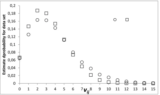
q2,2 using a random number (0-1) as input to the inverse accumulated Beta distribution and the parameters defined in Eqs. 5a or b. Secondly, the obtained values of p2,2 or q2,2 are used as input to Eq. 8a or 8b to draw a value of v2,2. The sequential procedure is repeated e.g. 10 000 times to make a set of v2,2 values. The results are shown in Fig. 4 using both

p2,2 (Eqs. 5a and 8a) and q2,2 (Eqs. 5b and 8b). Fig. 4 shows that the recorded value of v2,2 for any re-sampled data set of this size will be in the interval of 0-9 (or 10) visits, with 1-4 visits being the most likely values.

It is also possible to re-sample a whole data set and use these re-sampled data to test robustness of network descriptors calculated based on the data. The replication can be repeated thousands of times to find the percentile of the calculated descriptors, and the following example demonstrates how the ID method is easily applied for this purpose. The principle of the simulated re-sampling is to let the computer “sample” the data set: (1) Estimate the probability of “observing” a visit in the next sample for each combination of pollinator and plant species; (2) Use that probability to let the computer draw (decide) which combination to be sampled, as described in the text above Figure 4; (3) Repeat the item 1 and 2 until the number of data records is similar to the number in the original data set. The probability of “observing” a visit (Psi,j) is calculated as:

j i i j

i Q p

Ps, = ⋅ , 13

Where

Q

iis the probability of the simulated “observer” observing the pollinator species i without distinguishing between the plant species involved. The reasoning behind Eq. 13 is that the probability of observing the i’th pollinator species on the j’th plant species is equal to the probability of the i’th pollinator species to be observed as a visitor for any plant species and multiplied with the probability for the i’th pollinator to visit the plant species j when the pollinator species is observed. The Dirichlet distribution can be used to estimate the

Q

ivalue based on the V1,V2,⋅ ⋅⋅,Vi,⋅ ⋅⋅,VN values defined in Table 1. Instead of estimating the qi,jas the probability of pollinator species i to visit the plant species j , we are now estimating the probability of pollinator species i

to visit any plant species. So the principle of using the Dirichlet distribution remains for the merged data:

0 0,02 0,04 0,06 0,08 0,1 0,12 0,14 0,16 0,18 0,2

0 1 2 3 4 5 6 7 8 9 10 11 12 13 14 15

E

st

im

a

te

d

p

ro

b

a

b

il

it

y

fo

r

d

a

ta

s

e

t

v

_ij

Figure 4. Nested Monte Carlo estimation of the probability for getting different v2,2 values in a re-sampled data

set, where in total 53 recordings are made of pollinator species 2 (to estimate p2,2) and 14

recordings are made for plant species 2 (to estimate q2,2).

(

)

(

)

(

)

[

]

∏

( )

∏

=

=

⋅ + Γ

+ Γ

= N

i V j i N

i i

Vi

i Q V

N S f

1 ,

1 1

,V

Q ₁₄

where S is the total number of visits in the data set:

∑

= = N i

i V S

1

15 Where Q and V are the vectors: Q1,Q2⋅⋅⋅,Qi,⋅⋅⋅,QNand

N

i V

V V

V1, 2,⋅ ⋅⋅, ,⋅ ⋅⋅, respectively.

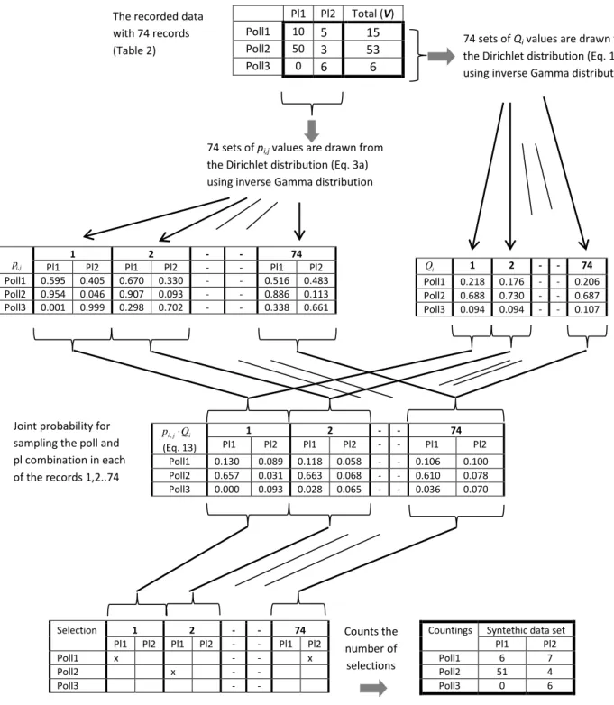
Thus, the probability of obtaining a record of the i‘th pollinator and the j’th plant species is a product of two probabilities, each being estimated by the data set using a Dirichlet distribution. It is possible to generate a random number that follows the Dirichlet distribution using an inverse Gamma distribution (see the algorithm in Frigyik et al. 2010). The principle of generating a single simulated data set, based on the Eqs. 3a, 13 and 14, is illustrated in Figure 5 for the data set in Table 2. The procedure in Figure 5 can be repeated to make a larger number of simulated data sets.

D

ISCUSSION

Clarification of governing assumptions for application of under-sampled data sets

The governing assumptions underpinning application of under-sampled data sets are evaluated using a conceptual model (Figure 1). This model can help to specify the type of probability that can be estimated based on the data depending on how the data are collected. An ideal data set is a random sample of visits without considering the pollinator or plant species, however, such a data set is difficult to obtain. If the governing assumption of sampling randomness is not fulfilled, then it conflicts with many descriptors that have been calculated based on the network analysis. Despite this, many cases of data collection are plant focused (Olesen et al. 2010) and this will only support the calculations of descriptors for each plant species separately. If the data are completely randomly sampled, then the ID method can estimate meaningful values for both q and p. However, in case of plant focused sampling, only q is meaningful, and in case of pollinator focused sampling, only p is meaningful. This problem of missing randomness should be consulted as a preliminary step before application of nearly any mutual network analysis method. This involves a careful description of the data collection protocols to display any form of potential bias. The conceptual model can help to clarify the usefulness of data set in network analysis by specifying the meaning of pollinator focused and plant focused data sets, respectively.

Assumptions underpinning the ID method

In plant-pollinator networks, some interactions never occur (termed forbidden links), for instance due to morphological and phenological mismatching (Jordano et al. 2003; Olesen et al. 2010). It may be well known that some pollinator species in the data set avoid visiting some plant species in the data set, and in this case it will improve the predictive power of the ID method to set the values in the

data set (Table 1) as “null”. The a priori assumption of the remaining “allowed” combinations of pollinator and plant species is that the plant species are equally likely to be visited by any allowable pollinator species, and all pollinator species are equally likely to visit any allowable plant species. This is described in Eqs. 6a and b, where the expectation for p and q

is 1/mi and 1/nj, respectively, if there are no records in the data set (Vi =Wj=0). The estimated probabilities can deviate more and more strongly from being equal distributed as the amount of data records increases.

A strength of the ID method is that, in contrast to other methods described in e.g. (Dormann et al. 2009), there is no need to assume any distribution of the data (log Normal or others) to be valid. Such additional assumptions open up for two types of uncertainties: (1) The structural uncertainty, where the form of the assumed distribution function may not be correct as description of the variability, e.g. it may allow nearly infinite high sampling values or more or less unknown truncations, (2) Parametric uncertainty, where the values of the distribution parameters (mean value, standard deviation etc.) may not be known for certain. This does not mean the ID method is always the best choice, as this depends on the condition of the data set and other sources of information in the particular case. If there are information available to parameterise and validate assumed distribution functions the statistical method as presented in (Dormann et al. 2009) could turn out to be as good or event better than the ID method. The ID method has a potential to be used especially when the validity of additional assumptions, others than given in the concept model, are insufficiently documented.

The ID method represents the simplest form for Bayesian approach, and in future activities it may be possible to develop more complex methods that better can take different type of a priori biological knowledge into account.

Methodological outcome as a contribution to better understanding

The ecological interpretation of p and q depends on the temporal and spatial scale of the data. If the data are collected over a few days in a local site where all pollinators have been foraging on the same plants and under more or less constant weather conditions, then p will reflect the real behaviour of the pollinators when they are choosing between different species of plants, and q will reflect a joint result of both pollinator abundance and behaviour. On the contrary, if the data are collected during a longer period, then some of the recorded plant species in the data set may not have been flowering synchronically during the investigation period (Olesen et al. 2010). In this type of data, a high pi,j value can either be due to the fact that plant species j is attractive compared to other plant species, or due to the fact that plant species j was the only one to blossom and, thus, to be visited during a critical period within the data collection. Similarly, a high qi,j value can be due to the fact that either plant species

j is attractive to pollinator species i compared to other pollinator species, or because pollinator species i was the only pollinator to be active during the flowering period of plant species j. For larger areas, the recorded pollinators may

Figure 5. Principle of resampling of 74 records to generate a synthetic data set on basis of the data set shown in Table 2. The original data set is used in the inverse Gamma distribution to draw stocastgically 74 set of respectively,

Q

iand pi,j values from their respective Dirichlet

distributions. The values of

Q

i and pi,j are multiplied (Eq. 13) and used to make a biased random selection of which pollinator to “sample”.

Thus, if

Q

1⋅

p

1,1= 0.130 then there is a 13.0 % change to “sample” the Poll1/Pl1 combination. Finally all the “synthetic” observations are

counted to yield the synthetic data set for 74 observations. not have been foraging in the same local area. In this case, the availability of plant species may not have been the same for different pollinator species, depending on their foraging radius and local abundance. In all cases, the values of p and q

disclose important ecological information, and the certainty of the estimates will show the statistical usefulness of the

under-sampled data for any quantitative interpretation. In all cases, the ID method can compile the data set to find statistical information about the interactions, but the interpretation of the results depends on the actual background of the data set.

i

Q 1 2 - - 74

Poll1 0.218 0.176 - - 0.206

Poll2 0.688 0.730 - - 0.687

Poll3 0.094 0.094 - - 0.107

Pl1 Pl2 Total (V)

Poll1 10 5 15

Poll2 50 3 53

Poll3 0 6 6

74 sets of pi,j values are drawn from

the Dirichlet distribution (Eq. 3a) using inverse Gamma distribution The recorded data

with 74 records (Table 2)

1 2 - - 74

Pl1 Pl2 Pl1 Pl2 - - Pl1 Pl2

Poll1 0.595 0.405 0.670 0.330 - - 0.516 0.483

Poll2 0.954 0.046 0.907 0.093 - - 0.886 0.113

Poll3 0.001 0.999 0.298 0.702 - - 0.338 0.661

i j i Q

p, ⋅

(Eq. 13)

1 2 - - 74

Pl1 Pl2 Pl1 Pl2 - - Pl1 Pl2

Poll1 0.130 0.089 0.118 0.058 - - 0.106 0.100

Poll2 0.657 0.031 0.663 0.068 - - 0.610 0.078

Poll3 0.000 0.093 0.028 0.065 - - 0.036 0.070

Selection 1 2 - - 74 Countings Syntethic data set

Pl1 Pl2 Pl1 Pl2 - - Pl1 Pl2 Pl1 Pl2

Poll1 x - - x Poll1 6 7

Poll2 x - - Poll2 51 4

Poll3 - - Poll3 0 6

Counts the number of selections

74 sets of Qi values are drawn from

the Dirichlet distribution (Eq. 14) using inverse Gamma distribution

Joint probability for sampling the poll and pl combination in each of the records 1,2..74

j i p,

The probabilistic property of respectively pi,j and qi,j makes them directly applicable for the entropy (Shannon) based indexes (Dormann et al., 2009). The ID method can, in contrast to existing approaches, generate synthetic data for construction of networks whiteout assuming any density function to govern the recorded number of visits (see Figure 5) and without assuming any fixed number of observations for pollinators and/or plants other than a fixed total number of records. The simulated data set can test any network calculation. e.g. the d’ and H2’ indexes suggested by (Blüthgen et al. 2006), using the real data set and many (more than 1 000) of the simulated data sets, respectively.

Application

The ID method has a general relevance for many resource-consumer networks for which the conceptual model (Fig 1) and data sets as defined in Tab. 1 apply. An add in for Excel 2010 and a related short tutorial, is made as supplementary material to this paper that runs the algorithm in Fig. 5. An empirical but close approximation to the invers gamma distribution is used in this add in to speed up the calculations and the add in will be continuously extended in the future. For all interested parties, it is possible to attend a mailing list by sending an e-mail to the first author of this paper. Definitely, software exists that can handle the Dirichlet distribution directly, e.g. Mathematica

(http://www.wolfram.com/mathematica/) or R

(http://www.r-project.org/).

A

CKNOWLEDGMENTS

This project was conceived and developed as part of STEP (Status and Trends of European Pollinators), which is funded by the European Commission as a Collaborative Project within Framework 7 under grant 244090 – STEP– CP – FP (Potts et al. 2011).

R

EFERENCES

Alarcón R, Waser N M, Ollerton J (2008) Year-to-year variation in the topology of a plant-pollinator interaction network. Oikos 117: 1796–1807.

Banašek-Richter C, Bersier LF, Cattin MF, Baltensperger R, Gabriel JP, Merz Y, Ulanowicz E, , Tavares AF, Williams DD, De Ruiter PC, Winemiller KO, Naisbit RE (2009) Complexity in quantitative food webs. Ecology 90: 1470-1477.

Bascompte J, Jordano P, Melián C.J, Olesen JM (2003) The nested assembly of plant-animal mutualistic networks. Proceedings of the National Academy of Sciences of the USA 100: 9383-9387. Bascompte J, Jordano P Olesen JM (2006) Asymmetric

coevolutionary networks facilitate biodiversity maintenance. Science 312: 431-433.

Biesmeijer JC, Roberts SPM, Reemer M, Ohlemüller R, Edwards M, Peeters T, Schaffers AP, Potts SG, Kleukers R, Thomas CD, Settele J, Kunin WE (206) Parallel Declines in Pollinators and Insect-Pollinated Plants in Britain and the Netherlands. Science 21:351-354.

Bersier LF, Banašek-Richter C, Cattin MF (2002). Quantitative descriptors of food web matrices. Ecology 83: 2394-2407. Blüthgen N, Menzel F, Blüthgen N (2006) Measuring

specialization in species interaction networks. BMC Ecology 6: 9.

Blüthgen N (2010) Why network analysis is often disconnected from community ecology: A critique and an ecologist’s guide. Basic and Applied Ecology 11, 185-195.

Dormann CF, Blüthgen N, Fründ J, Gruber B (2009) Indices, graphs and null models: Analyzing bipartite ecological networks. The Open Ecology Journal 2:7-24.

Dupont YL, Hansen DM, Olesen JM (2003) Structure of a plant - flower-visitor network in the high-altitude sub-alpine desert of Tenerife, Canary Islands. Ecography 26:301-310.

Dupont YL, Padrón B, Olesen JM Petanidou T (2009) Spatio-temporal variation in the structure ofpollination networks. Oikos 118:1261-1269.

Evans M, Hastings N, Peacock B (2000) Statistical Distributions (3rd ed.). Wiley Series in Probability and Statistics, John Wiley Sons, Inc.

Fortuna, M.A. &Bascompte, J. (2006) Habitat loss and the structure of plant–animal mutualistic networks. Ecology Letters 9: 281-286.

Frigyik BA, Kapila A, Gupta MR (2010) Introduction to the Dirichelt Distribution and Related Processes, UWEE Technical Report Number UWEETR-2010-0006.Department of Electrical Engineering, University of Washington.

Gibson RH, Knott B, Eberlein T, Memmott J (2011) Sampling method influences the structure of plant – pollinator networks. Oikos 120: 822-831.

Goldwasser L, Roughgarden J (1997) Construction and analysis of a large Caribbean food web. Ecology 74: 1216-1233.

Hegland SJ, Nielsen A, Lázaro A, Bjerknes AL, Totland Ø (2099) How does climate warming affect plant–pollinator interactions? Ecology Letters 12:184-195.

Ings TC, Montoya JM, Bascompte J, Bluthgen N, Brown L, Dormann CF, Edwards F, Figueroa D, Jacob U1, Jones JI, Lauridsen RB, Ledger ME, Lewis HM, Olesen JM, van Veen FJF, Warren PH Woodward G (2009) Ecological networks - beyond food webs. Journal of Animal Ecology 78: 253-269. Jordano P, Bascompte J Olesen JM (2003) Invariant properties in

coevolutionary networks of plant-animal interactions.Ecology Letters 6: 69-81.

Kaiser-Bunbury CN, Valentin T, Mougal J, Matatiken D Ghazoul J (2010) The tolerance of island plant–pollinator networks to alien plants. Journal of Ecology 99: 202-213.

Memmott J, Waser N, Price MV (2004) Tolerance of pollination networks to species extinctions. Proceedings of the Royal Society of London Series B 271: 2605-2611.

Memmott J, Craze PG, Waser NM, Price MV (2007) Global warming and the disruption of plant–pollinator interactions. Ecology Letters 10: 710-717.

Olesen JM Jordano P (2002) Geographic patterns in plant-pollinator mutualistic networks. Ecology 83: 2416-2424.. Olesen JM, Bascompte J, Dupont YL Jordano P (2006) The

smallest of all worlds: Pollination networks. Journal of Theoretical Biology 240: 270–276.

Olesen JM, Bascompte J, Dupont YL Jordano P (2007) The modularity of pollination networks. Proceedings of the National Academy of Sciences of the USA 104: 19891–19896.

Olesen JM, Bascompte J, Elberling H Jordano P (2008) Temporal dynamics in a pollination network. Ecology 89, 1573-1582. Olesen JM, Bascompte J, Dupont YL, Elberling H, Jordano P

(2010) Missing and forbidden links in mutualistic networks. Proceedings of the Royal Society of London Series B-Biological Sciences 278: 725-732.

Petanidou T, Kallimanis AS, Tzanopoulos J, Sgardelis SP Pantis JD (2008) Long-term observation of a pollination network: fluctuation in species and interactions, relative invariance of network structure and implications for estimates of specialization. Ecology Letters 11, 564–575.

Potts SG, Biesmeijer JC, Kremen C, Neumann P, Schweiger O, Kunin WE (2010) Global pollinator declines: trends, impacts and drivers. Trends in Ecology & Evolution 24:345-353.

Potts SG, Biesmeijer JC, Bommarco R, Felicioli A, Fischer M, Jokinen P, Kleijn D, Klein AM, Kunin WE, Neumann P, Penev LD, Petanidou T, Rasmont P, Roberts SPM, Smith HG, Sørensen PB, Steffan-Dewenter I, Vaissière BE, Vilà M, Vuji A, Woyciechowski M, Zobel M, Settele J and Schweiger O (2011)

Developing European conservation and mitigation tools for pollination services: approaches of the STEP (Status and Trends of European Pollinators) project. Journal of Apicultural Research 50:152-164.

Vazquez DP (2005) Degree distribution in plant-animal mutualistic networks: forbidden links or random interactions? Oikos 108: 421-426.

Vazquez DP, Aizen MA (2003) Null model analyses of specialization in plant-pollinator interactions. Ecology, 84:2493-2501.

Vázquez DP, Blüthgen N, Cagnolo L, Chacoff N P (2009) Uniting pattern and process in plant–animal mutualistic networks: a review. Annals of Botany 103: 1445–1457.