c
Sharif University of Technology, December 2009
Concurrent Project Scheduling and Material
Planning: A Genetic Algorithm Approach
M. Sheikh Sajadieh
1, Sh. Shadrokh
1;and F. Hassanzadeh
2Abstract. Scheduling projects incorporated with materials ordering results in a more realistic problem. This paper deals with the combined problem of project scheduling and material ordering. The purpose of this paper is to minimize the total cost of this problem by determining the optimal values of activity duration, activity nish time and the material ordering schedule subject to constraints. We employ a genetic algorithm approach to solve it. Elements of the algorithm, such as chromosome structure, untness function, crossover, mutation and local search operations are explained. The results of the experimentation are quite satisfactory.
Keywords: Project scheduling; Genetic algorithm; Material ordering.
INTRODUCTION
A traditional strategy was to treat project scheduling and materials ordering separately. Based on this strategy, project scheduling is rst carried out and, then by taking the activity schedule as a known parameter, a material ordering plan is determined. Following this method makes the project managers not consider the trade-os between cost elements such as material ordering costs, material holding costs, procurement costs and the reward or penalty for the project completion time and, therefore, the total cost of the project increases.
The rst paper in the integration of Project Scheduling and Material Ordering (PSMO) appears to be attributed to Aquilano and Smith [1]. They developed a model which integrates Material Require-ment Planning (MRP) consisting of material, lead-times and inventory level scheduling, and the Critical Path Method (CPM). Smith-Daniels and Aquilano [2] extended that work by proposing a heuristic procedure for scheduling large projects wherein requirements
1. Department of Industrial Engineering, Sharif University of Technology, Tehran, Iran.
2. Department of Computer Engineering, Ferdowsi University of Mashhad, Mashhad, Iran.
*. Corresponding author. E-mail: [email protected] Received 2 June 2007; received in revised form 17 February 2008; accepted 2 July 2008
for all renewable and non-renewable resources are incorporated. The heuristic also takes into account variations in activity duration and precedence con-straints.
Smith-Daniels and Smith-Daniels [3] presented a mixed integer programming model for a PSMO problem that oers an optimal scheduling of project activities and materials orders. They demonstrated that the latest starting time schedule provides an optimal solution. It was also shown that the problem can be solved optimally when it is decomposed into a derivation of the project schedule and a derivation of the materials ordering plan. They used the Wagner-Whitin algorithm [4] to nd the optimal ordering plan of materials for a known project schedule. Erabsi and Sepil [5] presented a heuristic procedure to determine the tradeo between expediting the materials ordering and delaying the project.
Dodin and Elimam [6] extended that work by including variable activity duration, variable project worth, rewards for early project completion and mate-rial quantity discounts into the model. They showed that the variability in activity duration gives more exibility to project scheduling, resulting in more cost reduction and allowing for savings on the completed activities and materials ordering cost. They formulated the problem as a mixed integer programming model and used some analytical results to reduce the size of the model and improve its solution eciency.
Compu-tational results show that solution times are strongly aected by the increase in problem size and, therefore, their numerical research was limited to the problems with 30 activities at the most.
Schmitt and Faaland [7] used a heuristic for scheduling a recurrent construction. The heuristic rst generates an initial schedule that dispatches worker teams to tasks for the backlogged products and, then, solves a series of maximal closure problems to nd material release times that maximize the net present value of cash ows.
In this paper, we extend the PSMO problem investigated by Dodin and Elimam [6] by developing a Genetic Algorithm (GA) approach to nd the optimal solution for large scale problems. The paper is orga-nized as follows. First, the modeling assumptions are discussed and expected cost functions are calculated. Then, the genetic algorithm approach is described. Fol-lowing that, numerical results and parametric analysis are presented. Finally, our ndings are summarized. PROBLEM DESCRIPTION
Assumptions
The following assumptions are used throughout this paper to develop the model:
1. A project with N activities is considered. The precedence relations of activities are zero-lag, nish-to-start and shown by an activity on the node net-work with no loop. Activities 1 and N are dummies that represent the project start and completion, respectively.
2. Activity duration is considered to be a variable that can vary from normal time to crash time.
3. The activities need M types of nonrenewable re-sources.
4. The amount required from material m to process activity j is independent of the activity duration. 5. All the amounts of each material needed for each
activity are ordered at the same time.
6. An all-unit discount policy is proposed for each material.
7. The objective function elements, which are pre-sented in the following section, are adopted from Dodin and Elimam [6].
Mathematical Model
The purpose of this paper is to minimize the total cost of the PSMO problem by determining the optimal values of activity duration, activity nish time and the material ordering schedule subject to constraints. We
use the same notation as introduced by Dodin and Elimam [6] for similar parameters as follows.
Indices
j = 1; ; N index of project activities, m = 1; ; M index of materials, k = 1; ; Km index of discount ranges,
t = 0; ; H index of time. Parameters
a. Activity related
Pj Set of activities preceding activity j,
bj Crashing cost of activity j,
cj The cost of reducing the duration of
activity j by one period,
uj Upper bound on the duration of activity j
(normal time),
vj Lower bound on the duration of activity j
(crash time),
ej The earliest completion time of activity j,
assuming that the project starts at time zero and the duration of each activity is equal to its crash time,
lj The latest completion time of activity j,
assuming that the project nishes at time H and the duration of each activity is equal to its crash time.
b. Material related
mk Limit on quantity range k of material m,
mk Cost of material m purchased in quantity
range k,
Gm Ordering cost of material m,
hm Inventory holding cost of one unit of
material m for one period,
Km Number of quantity discount ranges for
material m,
Lm Lead time of material m in periods,
Rjm Amount required from material m to
process activity j. c. Project related
d Due date of the project after which a delay penalty cost is paid,
H The planning horizon,
p Penalty cost per period for having the project late beyond d,
r Reward paid per period for completing the project before d,
s Percentage of the activity's worth representing the holding cost, per period, of the completed activities.
Non-Negative Variables: Xjt
(
1 If activity j is completed in period t. 0 Otherwise. Pmktj 8 > > > > > > < > > > > > > :
1 If mth material of activity j is ordered in period t and the total amount of orders in this period falls within quantity range k.
0 Otherwise. zj Duration of activity j:
mkt 8 > < > :
1 If material m is ordered within quantity range k in period t.
0 Otherwise.
Imt Inventory level of material type m by theend of period t.
wjt Worth of activity j completed by the end ofperiod t.
Wt Worth of project by the end of period t:
Model Formulation
The PSMO problem is formulated as a Mixed Integer Programming (MIP) model as follows:
minXN
j=1
[bj cj(zj vj)] d
X
t=eN
r(d t)XNt
+
H
X
t=d
p(t d)XNt H 1X
t=1
sWt
+XM
m=1 H LXm
t=1 Gm Km X k=1 mkt
+XM
m=1 H LXm
t=1 Km X k=1 N X j=1
mkRjmPmktj
+
M
X
m=1 H 1X
t=1
hmIm:
Subject to:
li
X
t=ei
tXit+ zj lj
X
t=ej
tXjt 0; 8i 2 Pj;
j = 1; ; N; (1)
X10= 1;
vj zj uj; j = 1; ; N; (2)
lj
X
t=ej
Xjt= 1; j = 1; ; N; (3)
wjt [bj cj(zj vj)] bj(1 Xjt);
j = 1; ; N; t = 1; ; H; (4)
Wt Wt 1+ N
X
j=1
wjt; t = 1; ; eN; (5)
W0= 0;
Wt Wt 1+ N
X
j=1
wjt
0 @XN
j=1
bj
1 A : Xt
=eN
XN;
t = eN + 1; ; H; (6)
Imt= Im(t 1)+ N X j=1 Rjm Km X k=1
Pmk(t Lm)j Xjt
! ;
m = 1; ; M; t = 1; ; H; (7)
Im0= 0; m = 1; ; M;
m(k 1)mkt N
X
j=1
RjmPmktj mkmkt;
m = 1; ; M; t = 1; ; H;
k = 1; ; Km; (8)
m0= 0; Km
X
k=1
mkt1; m=1; ; M; t=1; ; H;
(9)
Km
X
k=1 H 1X
t=1
Pmktj= 1; j = 1; ; N;
m = 1; ; M; (10)
Km
X
k=1 H 1X
t=1
tPmktj lj
X
t=ej
tXjt Lm;
j = 1; ; N; m = 1; ; M; (11)
Xjt= f0; 1g; mkt= f0; 1g;
zj 0; Imt 0; wjt 0; Wt 0;
8m; t; j: (13)
The total cost function consists of seven elements which are crashing cost, reward for early project completion, project delay penalty, completed activities holding cost, material ordering cost, procurement cost and inventory holding cost, respectively. Constraints 1 take into consideration the precedence relation between each pair of activities (i; j), where i immediately precedes j. Constraints 2 limit activity durations between their normal and crash time. Constraint 3 guarantees that each activity j can only have one nish time. Sets of Constraints 4-6 are used to calculate activities and project worth. Constraint 7 is a balance equation to monitor the inventory level over the planning horizon. Constraints 8 and 9 satisfy the discount conditions, where the order quantity from each material per period should be in an appropriate interval of the discount pricing schedule and only in one interval. Constraint 10 guarantees that each material m is ordered for each activity j just one time. Constraint 11 stipulates that all materials required for each activity should be ready at the activity nish time. The sets of Constraints 12 and 13 denote the domain of variables.
One can convert the problem to a multidimen-sional 0-1 knapsack problem (Freville [8]). For ex-ample, if we simplify the model by assuming the activity duration to be constant, then Constraints 4 to 6, which are used to linearize the model, can be omitted and, thus, PH 1t=1 sWt will be replaced with
PN
j=1s(bj cj(zj vj))(PHt=1tXNt PHt=1tXjt) in
the objective function. Now, if we relax all constraints except Constraints 1, 3 and 11 and also reduce the objective function to just minimizing the completed activity holding cost, then we reach the following model:
minXN
j=1
s(bj cj(zj vj)) H
X
t=1
tXNt H
X
t=1
tXjt
! ; st:
li
X
t=ei
tXit+ zj lj
X
t=ej
tXjt 0; 8i 2 Pj;
j = 1; ; N;
lj
X
t=ej
Xjt= 1; j = 1; ; N;
Km
X
k=1 H 1X
t=1
tPmktj lj
X
t=ej
tXjt Lm; j = 1; ; N;
m = 1; ; M;
Xjt= f0; 1g; 8j; t:
This is a multidimensional 0-1 knapsack model, which is a known NP-hard. Since PSMO can be converted to an NP-hard problem with some simplication, so PSMO is also NP-hard. Thus, the optimal solution can only be achieved by exact algorithms in small instances. Therefore, heuristic methods are needed to solve large scale problems. We propose a genetic algorithm to solve the problem. However, one may compare the results of GA with other heuristic methods in order to clear up which one is more ecient.
GENETIC ALGORITHM Basic Scheme
One of the most important aspects of the genetic algorithm is the structure of its chromosomes (Geno-type), which is explained in the following section. Each chromosome gives a unique value to the decision variables, which are activity durations (zj's), activity
nish times (fj's) and the ordering times of materials
(otmj's). The following is a presentation of the scheme
of the algorithm.
The genetic algorithm starts by the random gen-eration of the initial population and by computing its untness, which is the cost of its related schedule. The size of the population, P S = 100 (N M), remains
constant for all generations. Each new generation is made from existing generations using three operations: crossover, mutation, and local search. In the crossover operation, Pcr percentages of pairs of parents are
randomly selected from the existing generation and, on each pair, a crossover operation is performed. Additionally, Pmu percentage of individuals, randomly
selected, is considered for mutation operation. More-over, a local search operation is employed to improve some randomly selected individuals. A local search is used for Pl percentage of individuals. The number of
individuals generated by each run is assumed to be equal to P S and, thus, 2Pcr+ Pmu+ Pl= 1.
After constructing each generation by the above operations, we choose the members of the next gen-eration by retaining the best Pse percentage of the
previous generation and selecting the remaining 1 Pse
percentage with transference rule.
The termination criterion is set as 150 generations with no improvement in the best solution. If this condi-tion has been satised, then the GA stops and returns the best individual. Otherwise, a new generation will
be generated. Note that , Pcr, Pmu, Pl and Pse are
adjustable parameters of the algorithm. Chromosome Representation
Each individual, I, is constructed from a (M + 2) N matrix. The rst row of this matrix represents activity durations. The second row represents activity nish times and the third to (M + 2)th rows represent the ordering times of materials for each activity. Based on the model, all of these cells contain integer values.
I = 2 6 6 6 6 6 6 6 6 6 6 6 6 4
zI
1 z2I zIN
fI
1 f2I fNI
otI
11 otI12 otI1N
otI
M1 otIM2 otIMN
3 7 7 7 7 7 7 7 7 7 7 7 7 5 :
Considering DVI
mq to be the qth set of activities in
chromosome I where their mth material is ordered in the same time, and DVI
mto be the number of dierent
sets of similar otI
mjin the ordering schedule of material
m, the value of untness function, f(I), would be f(I) = P7
i=1 I
i, so that:
I 1=
N
X
j=1
[bj cj(zIj vj)];
I
2= r(d fNI); if fNI d;
I
3= p(fNI d); if fNI > d;
I 4= s
N
X
j=1
[bj cj(zjI vj)](fNI fjI);
I 5=
M
X
m=1
GmDVmI;
I 6=
M
X
m=1 DVI
m
X
q=1
0
@ X
m2DVI mq
Rjm
1 A mk;
if m(k 1)
0
@ X
m2DVI mq
Rjm
1
A mk;
k = 1; ; Km;
I 7=
M
X
m=1 N
X
j=1
hmRjm(fjI otImj Lm):
Initial Population
We generate the initial population using two ap-proaches. Creating initial population members in these ways ensures that all chromosomes in the initial population represent feasible solutions. The detailed design of each code follows:
(a) Forward approach
The pseudo-code of this approach is given below: A= set of activities that can be selected (their
precedence activities have been selected be-fore).
P Ni= number of precedents of activity i that
have not been selected yet. Set j = 1
While j N
zj int [vj; uj], a discrete uniform
distribution, including vj and uj
j j + 1 End while
Set A = f1g, j = 1, f1= 0, P Ni=
X
k2Pi18i
While A 6=
Select one activity from A by random (e.g. j) fj maxi2P
jffig + zj
P Ni P Ni 1 8ijj 2 Pi
P Nj 1
A A fjg + f8ijP Ni= 0g
End while Set m = 1, j = 1 While m M
While j N
otmj int [0; fj Lm]
j j + 1 End while
Set j = 1, m m + 1 End while
(b) Backward approach
This approach is almost similar to the forward ap-proach, except that we start from H coming back to zero and, after generating the chromosome, all activities are locally shifted so that the start time of the project is equal to zero.
Crossover Operator
We use three crossover operators: one-point, two-point, and three-point crossovers. Let P a1 and P a2be a pair
of parents selected for crossovers. Two children, I1and
I2, are dened from this crossover. The pseudo-code of
the one-point crossover operator is given below: I1 P a1, I2 P a2
r int [2; N 1], selecting a breaking point Set k = 1
While k 2
Set lf = H, j = r + 1 While j N
Set mf = 0, i = 0 While i r
If i 2 Pj & fiIk> mf then mf fiIk
i i + 1 End while If fIk
j zIjk mf <lf then lf fjIk zIjk mf
j j + 1 End while
If lf > 0 then lf int [0; lf] fIk
j fjIk lf 8 j r + 1
Set j = r + 1 While j N
otIk
mj otImjk lf + a 8m
If otIk
mj< 0 then otImjk int [0; fj Lm]
j j + 1 End while k k + 1 End while
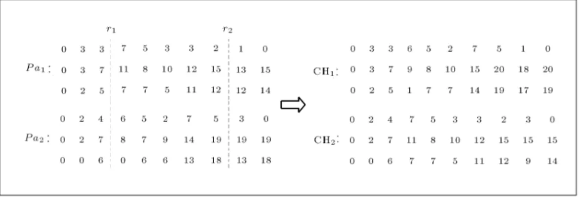
The second and third crossover operators use the same logic. For example, if in a two point crossover, P a1and P a2are a pair of parents selected for crossover,
then CH1and CH2will be their child, assuming r1and
r2as breaking points (Figure 1).
Mutation Operator
We use two mutations. Let I be the chromosome that is selected for mutation. The rst mutation operator selects = N=5 integer numbers randomly from the interval [2; N 1], representing selected activities, and an integer number, m, from the interval [1; M]. Then, a new ordering time of the selected material is generated for selected activities. Using this operator, activity durations and nish times remain unchanged. The pseudo-code of this operator is as follows:
N=5 Set a = 1 While a
j int[2; N 1] m int[1; M] otI
mj int[0; fjI Lm]
a a + 1 End while
The second mutation selects = N=5 integer numbers randomly from the interval [2; N 1], representing activities, and replaces the selected activity's duration by a new random value. Thus, activity nish times and ordering times may need change. We use the approaches employed for initial population generation to update the second to the (M + 2)th rows. The pseudo-code of this operator is as follows:
N=5 Set a = 1 While a
Figure 1. Two-point crossover example.
j int [2; N 1] zI
j int [vj; uj]
a a + 1 End while
Update fI and otI, using forward or backward
ap-proach.
Local Search Operator
Applying a local search, we are trying to change from existing chromosomes to those with less untness, by increasing the ordering times uniformity. This results in less ordering costs. Moreover, higher discount ranges may be achievable and thus, total cost may decrease. Two local search operators are employed in the algorithm. Considering as the selected chromosome for a local search, the pseudo-code of the rst operator is as follows:
N:M=10 Set a = 1 While a Nf H
m int [1; M], selecting a material
s = s0 int [2; 5], number of activities whose
ordering time will be the same j = j0 int [s; N]
While s 1, obtaining minimal potential ordering time
If fI
j Lm Nf then Nf fjI Lm
j j 1, s s 1 End while
While s0 1, replacing new ordering times
otI
mj0 Nf
j0 j0 1, s0 s0 1
End while a a + 1 End while
The second operator is almost the same as the rst except that those activities whose ordering times should become similar are selected randomly.
Transference Rule
Using the transference rule, the next generation of chro-mosomes is chosen from the list of existing individuals. This way, we rst obtain #I = f(I)= maxIf(I) and
then, a random value is generated between (0; #I) for
each individual. The individuals with fewer values are selected for the next generation.
COMPUTATIONAL RESULTS
Computational studies on the proposed GA for the PSMO problem have been carried out. The purpose of these experiments was to evaluate the performance of our GA across a variety of situations. To test the proposed GA, we developed experiments for networks with 10, 30, 60, 90 and 120 non-dummy activities and 1 to 4 materials. The structure of the networks as well as activities' normal duration was generated using
ProGen software [9]. The remaining input parameters were generated at random from a set of parameters; one for each of the underlying parameters.
All of the computations were performed on an IBM-compatible PC with Pentium 4 and 2.80 GHz, CPU speed and 512 MB RAM memory under Windows XP as the operating system. All procedures have been coded in C++ and compiled with the Microsoft Visual C++ 6.0 compiler.
Parameter Setting
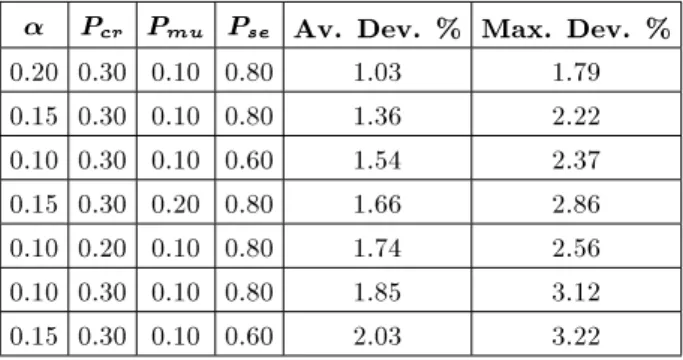
In order to improve the performance of GA, we use the design of experiment techniques to nd the good GA set of parameters before running the GA. The prelim-inary tests were conducted to determine appropriate values for , Pcr, Pmu and Pse. The experimental
layout is a full-factorial design [10], involving four factors. This experimental layout used three levels for each factor. The following selections for the parameter values are used: 2 f0:10; 0:15; 0:20g, Pcr 2 f0:1; 0:2; 0:3g, Pmu 2 f0:1; 0:2; 0:3g and Pse 2
f0:4; 0:6; 0:8g. Each row of experimental runs is one combination of these factors and, hence, there are 81 rows. In each row, we run the GA for 4 seconds for 10 certain instances with 60 non-dummy activities and four resources. Thus, 810 instances were solved. We used the average of 20 runs of each instance for the parameter setting. The distribution of these average values is needed for statistical analysis. Using the Shapiro-Wilk test, the assumption of normality distribution was strongly supported.
The average and maximum percent deviation from minimal cost, among all combinations of param-eter, were calculated for each row. Using the Duncan Multiple Range test with a signicance level equal to 0.05, we see that there are no signicant dierences between levels of Pse.
Table 1 shows some of the good combinations of parameter values and their results with 4-second computing time.
After the test, it was determined that the best results can be obtained by setting 0.2, 0.3, 0.1 and 0.8 for , Pcr, Pmu and Pse, respectively. Based on the
relationship between Pcr, Pmu and Pl, the best value
of Pl will be 0.3.
Table 1. Good combinations of parameter values. Pcr Pmu Pse Av. Dev. % Max. Dev. %
0.20 0.30 0.10 0.80 1.03 1.79 0.15 0.30 0.10 0.80 1.36 2.22 0.10 0.30 0.10 0.60 1.54 2.37 0.15 0.30 0.20 0.80 1.66 2.86 0.10 0.20 0.10 0.80 1.74 2.56 0.10 0.30 0.10 0.80 1.85 3.12 0.15 0.30 0.10 0.60 2.03 3.22
Performance Analysis
For an analysis of the performance of the GA, 12 instances with 10 activities and 1 to 4 resources were generated and tested. The parameters obtained from the parameter setting step (the previous section) are used for further GA runs. Table 2 shows the results of comparing optimal solutions attained by LINGO 8.0 with the solutions proposed by GA.
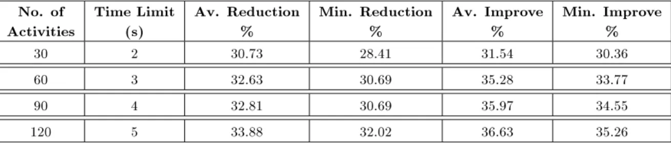
We also compared the solutions obtained from GA with the best randomly generated solutions after a time limit. Moreover, for testing the eciency of the GA, the best solution of the initial population is compared with the best solution found by the algorithm after a time limit. We generated 80 instances with 30, 60, 90 and 120 activities and 1 to 4 materials. The following measures are calculated:
Reduction % = 100 (BI BA)=BI; Improve % = 100 (BR BA)=BR;
where BR, BA and BI are best random solutions, the best solution found by the algorithm, and the best solution of initial population, respectively.
Table 3 shows that the algorithm improves the best untness value obtained from the initial pop-ulation and random generation by 32.51 and 34.85 percentages on average, respectively.
The Eect of Local Search
In order to test the eect of local search, 80 instances were generated. We obtained the best untness values with and without a local search after a certain time
Table 2. GA vs. optimal results. No. of
Activities
No. of Materials
LINGO CPU Time (s)
GA Av. CPU Time (s)
Av. Dev. %
Max. Dev. % 10 1 36.7 0.27 0.27 0.93 10 2 133.3 0.66 0.97 2.09 10 3 604.7 1.02 1.50 2.52 10 4 2462.0 1.64 1.88 2.85
Table 3. GA vs. random and initial values. No. of
Activities
Time Limit (s)
Av. Reduction %
Min. Reduction %
Av. Improve %
Min. Improve % 30 2 30.73 28.41 31.54 30.36 60 3 32.63 30.69 35.28 33.77 90 4 32.81 30.69 35.97 34.55 120 5 33.88 32.02 36.63 35.26
Table 4. Eect of local search. No. of
Materials
Time Limit (s)
Average Percent Improvement % 1 2 5.66 2 2 5.84 3 2 14.45 4 2 19.14 1 3 5.29 2 3 16.13 3 3 20.75 4 3 29.59 1 4 12.05 2 4 21.49 3 4 26.12 4 4 27.51 1 5 10.48 2 5 24.59 3 5 31.77 4 5 34.67
limit. The parameters of the GA without the local search are: = 0:2, Pcr = 0:4, Pmu = 0:2 and
Pse = 0:8. Considering FL and FWL to be the best
untness values for the algorithm with and without a local search, the percentage improvement is dened as 100 (FWL-FL)/FWL. The average improvement for each set of problems is shown in Table 4.
CONCLUSION AND DIRECTIONS FOR FUTURE RESEARCH
A model was developed to integrate the problem of project scheduling with material ordering. This paper is an extension of the PSMO problem investigated by Dodin and Elimam [6] by developing a solution approach so that the model can be solved for large scale problems. The problem is formulated as a Mixed Integer Programming model and a genetic algorithm approach is employed to solve the problem. Finally,
the performance of the algorithm was evaluated by solving dierent instances so that the results were quite satisfactory.
One of the future research directions is to extend this study for stochastic supply lead-times in which the objective function is to minimize the expected total cost per unit time. Other discount policies can also be considered as an extension.
REFERENCES
1. Aquilano, N.J. and Smith, D.E. \A formal set of algorithms for project scheduling with critical path method-material requirements planning", J. of Oper. Manag., 1(2), pp. 57-67 (1980).
2. Smith-Daniels, D.E. and Aquilano, N.J. \Constrained resource project scheduling subject to material con-straints", J. of Oper. Manag., 4(4), pp. 369-388 (1984). 3. Smith-Daniels, D.E. and Smith-Daniels, V.L. \Opti-mal project scheduling with materials ordering", IIE Trans., 19(4), pp. 122-129 (1987).
4. Wagner, H.M. and Whitin, T.M. \Dynamic version of the economic lot size model", Manag. Sci., 5(1), pp. 89-96 (1958).
5. Erabsi, A. and Sepil, C. \A modied heuristic proce-dure for materials management in project networks", Int. J. of Ind. Eng.-Theory, 6(2), pp. 132-140 (1999). 6. Dodin, B. and Elimam, A.A. \Integrated project
scheduling and material planning with variable activity duration and rewards", IIE Trans., 33, pp. 1005-1018 (2001).
7. Schmitt, T. and Faaland, B. \Scheduling recurrent construction", Naval Res. Logist., 51(8), pp. 1102-1128 (2004).
8. Freville, A. \The multidimensional 0-1 Knapsack prob-lem: An overview", Eur. J. Oper. Res., 155, pp. 1-21 (2004).
9. Kolisch, R., Sprecher, A. and Drexl, A. \Character-ization and generation of a general class of resource-constrained project scheduling problems", Manag. Sci., 41, pp. 1693-1703 (1995).
10. Montgomery, D.C., Design and Analysis of Experi-ments, 4th Edn., John Wiley & Sons (1996).