Sharif University of Technology
Scientia IranicaTransactions E: Industrial Engineering www.scientiairanica.com
A particle swarm optimization-based algorithm for
exible assembly job shop scheduling problem with
sequence dependent setup times
S. Nourali
a;1;and N. Imanipour
ba. Faculty of Management and Accounting, Department of Industrial Management, Islamic Azad University, South Tehran Branch, Tehran, Iran.
b. Faculty of Entrepreneurship, University of Tehran, Tehran, Iran.
Received 15 October 2012; received in revised form 6 May 2013; accepted 15 July 2013
KEYWORDS Flexible job shop scheduling; Assembly;
Sequence dependent setup time;
Particle swarm optimization.
Abstract. This paper considers a exible assembly job shop scheduling problem with sequence dependent setup times, and its objective is the minimization of makespan, which integrates the process planning and scheduling activities. This is a combinatorial optimization problem with substantially large solution space, suggesting that it is highly dicult to nd the best solution with the exact search method. In this paper, a particle swarm optimization based algorithm is proposed, which applies a novel solution representation method to t the continuous nature of the algorithm in the discrete modeled problem. Numerical experiments also have been performed to demonstrate the eectiveness of the proposed algorithm.
c
2014 Sharif University of Technology. All rights reserved.
1. Introduction
Nowadays, manufacturing systems have to produce orders in minimum time in order to increase their competition capability in the market. Production scheduling is one of the factors to play a direct, basic role in achieving this goal. The development of advanced techniques in this eld of science, thus, is one of the issues considered by researchers. Flexibility is also an obvious characteristic of modern manufacturing systems, which is another factor towards attaining the mentioned goal. Various denitions of exibility in manufacturing systems can be found in the literature. Benjafaar and Ramakrishman [1] divided exibility into two main groups. The rst group considers 1. Iran Water Resources Management Co., No. 517, North
Felestin Street, Tehran, Iran.
*. Corresponding author. Tel.: +98 9125038497; Fax: +98 21 88891959
E-mail addresses: st s [email protected] (S. Nourali); [email protected] (N. Imanipour)
exibility in the process of production. Flexibility, with respect to processes implicates conditions under which machines have the capability of implementing more than one operation. The second group also explains exibility with respect to production. This group itself is divided into three sub-groups. Oper-ation exibility is considered when there are several alternative machines for implementing an operation (sometimes this condition is named, routing exibility). Sequencing exibility refers to conditions in which there are several alternative plans for the operation sequence of a job (this condition is sometimes named, process plan exibility).
Moreover, processing exibility is a condition, under which, in addition to existing alternative opera-tion sequences for each job, there are various types of operation in the process plans.
In traditional approaches, the process planning activity is performed independent of scheduling activ-ity. In other words, the relation between these two activities is completely unilateral, and the scheduling
activity is performed by considering certain and pre-determined process plans. The separation of process planning and scheduling activities may cause some disadvantages. Each one of these activities searches a vast solution space for nding a good solution. If a process plan is not implemented in the scheduling phase, eorts made to nd it would be aborted. Con-versely, integration of process planning and scheduling activities provides a unique solution space (however, more complex). Thus, if two activities are integrated successfully, a considerable saving occurs in costs re-lated to solving the problem [2].
In the literature, the above problem is usu-ally named the Integration of Process Planning and Scheduling (IPPS) problem. An IPPS problem is also known as the Flexible Job Shop Scheduling (FJSS) problem. In fact, any kinds of FJSS problem can be seen as an IPPS problem. Over the past decade, dierent approaches have been proposed for solving the problem. As for the shop oor status, Jain et al. [3] divided the approaches into two main groups. The rst group includes approaches that perform integration dynamically. In other words, these approaches focus on shop oor conditions to perform the process planning activity. Sometimes, these types of method are divided into two sub-groups; closed loop process planning [4] and distributed process planning [5]. In contrast, the second group includes methods which consider the status of the shop oor to be fully static and are named Non-Linear Process Planning (NLPP). This approach implicates situations in which all possible process plans for a job are designed before application to the shop oor. On this basis, the process plans for each job are prioritized based on specic criteria. During the production process, the process plan with the highest priority is always considered as the rst option for utilization in the workshop. If the conditions are not favorable for use, subsequent priorities will be considered.
Jain et al. [3] investigated some advantages and disadvantages of the mentioned approaches and con-cluded that the second approach (i.e. NLPP) can be a fair tool for IPPS, and can be utilized in plants where there are separate departments for process planning and scheduling without any changes in their organiza-tion. Moreover, using this approach in order to utilize exibility, they proposed a methodology, which, due to its simplicity, is included in most current research. The integration model focuses on the implementation and improvement of this model [6].
Considering the NLPP approach, a vast range of research has been undertaken in past years which could be classied into two groups, according to the problem solving method: I) exact solutions, and II) metaheuristics.
Regarding the rst group, Tan and Khoshnevis [7]
proposed a polynomial mixed integer programming model for the IPPS problem and linearized it. Ozguven et al. [8] presented a mixed integer linear programming model for solving this problem; they rst proposed a new model for the Flexible Job Shop Scheduling problem with routing exibility and compared it with the only comparable model they found in the literature. Afterwards, this model was developed considering pro-cess plan exibility.
Because of the diculty in solving combinatorial optimization problems in real-size by an exact method, most studies on the IPPS problem focused on the use and development of meta-heuristics to nd high quality solutions for the problem. In a review study, Tan and Khoshnevis [2] investigated the capability of development of various methods to solve the mentioned problem. The study was focused on introducing process planning systems based on articial intelligence. Ima-nipour et al. [9] modeled the problem as a non-linear mixed integer programming model with the objective of minimizing maximum lateness, and solved it by two new versions of the tabu search algorithm. They also considered transportation times in their model. Ima-nipour [10] proposed a non-linear mixed integer pro-gramming for the IPPS problem considering sequence dependent setup times and developed a tabu search algorithm to solve the problem. Li and McMahon [11] proposed an approach based on the simulated anneal-ing algorithm in order to solve the IPPS problem. Moon and Seo [12] developed a mathematical model for solving the problem in a multi plant chain, considering transportation times. In addition, they presented an evolutionary algorithm for solving the proposed model. Moon et al. [13] presented a mixed integer programming model and an evolutionary algorithm, based on a topological type, to solve the IPPS problem in a supply chain. Guo et al. [14] used a modied Particle Swarm Optimization (PSO) algorithm to solve the problem in single objective mode. Shao et al. [15] proposed a modied approach based on the genetic algorithm for the IPPS problem. Li et al. [6] proposed a new hybrid algorithm to solve the problem. They devised a collection of new genetic representations and genetic operators in the algorithm. They also used the tabu search algorithm for local search. In addition, Li et al. [16] presented a mathematical model for the IPPS problem and proposed an evolutionary based algorithm to solve it. Wang et al. [17] proposed a new solution representation to use in the PSO algorithm for this problem and devised a local search approach to improve solution quality.
Nourali et al. [18] recently proposed a new math-ematical model for the IPPS problem. They compared the literature of the IPPS problem with the assembly job shop scheduling problem and concluded that the assembly operation is a neglected issue regarding the
IPPS problem. So, they dened a new problem, entitled the Flexible Assembly Job Shop Scheduling (FAJSS) problem, which included the assumptions of the IPPS problem with the addition of assembly operation. They proposed a mixed integer linear programming model to minimize makespan for the problem, considering sequence dependent setup times, and solved it using only a branch and bound method. As mentioned above, it is very dicult to solve such a problem by an exact method in real size problems. So, it is required to develop a powerful approximate algorithm for searching the large solution space of the problem.
This paper considers the new problem addressed by Nourali et al. [18]. However, the major aim is to develop an ecient meta-heuristic algorithm based on PSO to nd good solutions for large size problems that cannot be solved optimally by an exact solution in reasonable time. The algorithm applies a new solution representation method for this problem, which is the second achievement of this paper. Problems of various sizes are also used to test the performance of the proposed algorithm. The rest of this paper has been organized as follows: Section 2 is devoted to the denition of the problem. In Section 3, the PSO algorithm is introduced. Section 4 describes the proposed algorithm and its components. Section 5 discusses computational results and, nally, Section 6 includes the concluding remarks and future research. 2. Problem denition
Based on the denition presented by Nourali et al. [18], \job" refers to a nal product which is composed of some \parts". The parts are assembled, based on predecessor/successor relationships, according to the bill of materials, to form a nal product or a job. An example is shown in Figure 1. In this gure, each rectangle represents a part. The parts have been labeled with ij, which means the jth part of job i. The part, ij, may be a root component, a leaf component or a subassembly of a job. In this gure, part 10 is a root component, parts 11, 13 and 14 are leaf components, and part 12 is a subassembly of job 1. It is assumed that part i0 represents the nal assembly for job i and can be considered the nal product. Each part requires a set of determined operations, which are shown in Figure 1 using circles. There are predened relationships between the operations of each part. All the scenarios of exibility mentioned in Section 1 are considered in the problem. The processing times of the operations are dierent and deterministic in the alternative machines. The setup times of the operations are dierent and sequence dependent. When the processing part is changed, setup would be required for the machine. In other words, if
Figure 1. Predecessor/successor relationships for a job with 5 parts.
the operations of a particular part are processed by a machine successively, setup will not be required.
Generally, in classical job shop scheduling prob-lems, a job is considered a batch of identical jobs. Mckoy and Egbelu [19] indicated that this strategy leads to an increase in Makespan. Therefore, in this paper, similar parts are considered as distinct parts. It is assumed that the setup time between these parts is equal to zero. It is expected that this assumption will lead to maximum utilization of exibility on the shop oor.
Some other assumptions and constraints are de-scribed as follows:
Cutting operation is not permitted.
A part can only be processed on one machine at a time, and a machine can process only one operation at a time.
Transportation times are ignored.
All parts are available at time zero.
During the time horizon of the schedule, machines are available and are not broken.
A dummy job is also considered which has only one part. The number of operations of this part is equal to the number of existing machines in the workshop and each operation is performed by only one machine. All processing times related to this part are equal to zero. This part is assumed in order to consider the rst setup on the machines. In other words, the part which is processed immediately after the dummy job could be considered the rst processed part on the machine.
The aim is to generate a schedule which mini-mizes the makespan, considering all technological and resources constraints. (Note that the makespan is calculated in terms of the completion times of nal
products or jobs.) The mathematical formulation of the problem can be found in Nourali et al. [18]. 3. Particle swarm optimization
The PSO algorithm was introduced by Kennedy and Eberhart [20]. This algorithm, which is designed based on the simulation of the social behavior of birds in a ock, was originally adopted for balancing weights in neural networks. The PSO algorithm is an evolutionary algorithm that starts with an initial population of randomly generated individuals, named a swarm. Each particle in this algorithm indicates a feasible solution from the solution space. The particles search the solution space by velocities which are calculated at each step of the algorithm. Eqs. (1) and (2) are the most popular relations for updating the velocity and position vectors of the particles in the PSO algorithm:
~vi(t + 1) = [W:~vi(t)] +
h r1:c1:
~xipbest ~xi(t)
i
+
r2:c2:
~xgbest ~x i(t)
; (1)
~xi(t + 1) = ~xi(t) + ~vi(t + 1): (2)
In this algorithm, the best position vector found by each particle is reserved in ~xipbest, where i is a counter
for the particles. Also, the best position vector found by the entire swarm is reserved in ~xgbest. These
posi-tions are considered as leaders for the next movement of a given particle. The velocity vectors are updated by Eq. (1), where W is the inertia weight. Researchers have found that the best performance can be obtained by initially setting W to some relatively high value, which corresponds to a system where the particles move in a low viscosity medium and perform extensive exploration, and gradually reducing W to a much lower value, where the system would be more dissipative and exploitative and would be better at homing in to local optima [21]. In Eq. (1), c1, which is named the
cognitive learning factor, indicates the learning rate of each particle from the best solution it has found. Also, c2, which is named the social learning factor,
indicates the learning rate of each particle from the best solution found by the entire swarm. The value 2 has been adopted for these parameters in most research on the PSO algorithm. Parameters, r1 and r2, are
also randomly generated gures within the range [0,1], which are used to maintain diversity in the search process.
4. The proposed algorithm
To solve the FAJSS problem with the sequence depen-dent setup times, three sub-problems should be solved
simultaneously: (I) selecting the most suitable process plan for each part, (II) assigning the most suitable machines for the operations, (III) determination of the best schedule.
In order to solve these problems simultaneously, it is required to combine their solution spaces. This combination is resulted to produce a complicated solu-tion space. The proposed algorithm has been designed in such a way as to be able to search this vast solution space ideally.
4.1. General structure
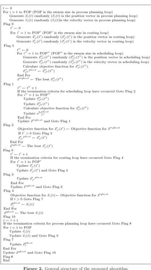
The general structure of the proposed algorithm can be found in Figure 2. The algorithm consists of three nested loops. The duty of the outermost loop is to nd the most suitable process plans for the parts, which, hereinafter, will be named the \process planning loop". The middle loop is recalled in the process planning loop, and its duty is to assign the most suitable machines for operations, with respect to the selected process plans in the process planning loop. Henceforth, this loop is named the \routing loop". The innermost loop, which is recalled in the routing loop, is responsible for determination of the best schedule, with respect to the outputs of two outer loops. This loop is named the \scheduling loop".
Each loop searches the solution space based on the concepts of the PSO algorithm mentioned in Section 3. At rst, a particle from the process planning loop is initialized randomly and the process plan for the parts is determined. This process plan is considered the input for the routing loop. Then, a particle from the routing loop is initialized randomly, with respect to the selected process plan, by the process planning loop to assign machines to the operations. Afterward, the outputs of these two loops are considered as the input of the innermost loop, i.e. the scheduling loop. In this loop, the rst particle is initialized randomly with respect to the outputs of other loops, and the rst schedule is produced for the problem. Based on this schedule, the objective function value is calculated for the rst time. This value is considered the objective function value for the rst particle of the scheduling loop. Afterwards, the scheduling loop initializes its other particles and calculates their objective function value. In order to nd the most suitable schedule for the selected process and routing plans, the scheduling loop begins iterations, according to Eqs. (1) and (2), and until the occurrence of termination criteria of this loop, the process continues.
When the scheduling loop is terminated for the rst time, the best schedule found by this loop is considered the objective function value for the rst particle from the routing loop. Then, the second particle from the routing loop is initialized randomly and new information is reported to the scheduling loop
Figure 2. General structure of the proposed algorithm.
again. Afterwards, the scheduling loop is recalled, as before, to nd the most suitable schedule, with respect to the selected process plan and new selected routing plan. The process is continued until all the particles from the routing loop are initialized. After initializing, the routing loop begins iterations, based on Eqs. (1) and (2), like the scheduling loop. After the termination
of the routing loop, the best objective function value found by this loop is considered the objective function value for the rst particle from the process planning loop. The process planning loop also acts like the other loops. After the termination of the process planning loop, the best solution found by this loop is considered the best schedule for the problem.
As mentioned at the beginning of this section, in order to solve the sub-problems simultaneously, it is necessary to combine their solution space, which results in an increase in the complexity of problem solving. The advantage of the proposed structure of this paper is to choose a part of the solution space at each stage, and search therein, in order to nd the best solution.
In such a way, it would be expected to search the vast solution space of the problem favorably.
4.2. Solution representation method
Originally, the PSO algorithm was designed to solve continuous problems. Lei [22] addressed two ap-proaches in the literature for applying this algorithm in discrete problems, such as the job shop scheduling problem. In the rst approach, named discrete PSO, the position or velocity update method is redened to apply in discrete problems. The redenition is essential for the application of PSO. On the other hand, the low performance of the discrete PSO mainly results from its redenition. This is a paradox [22]. The second approach is to transform the discrete problem into a continuous one. By this approach, it is not required to redene the elements of the PSO algorithm. Lei [22] enumerated the advantages of the second approach and concluded that the transformation of a discrete problem into a continuous one is much easier than redenition of the elements of the PSO algorithm. In this study, the second approach has been adopted and the problem has been converted into a continuous problem.
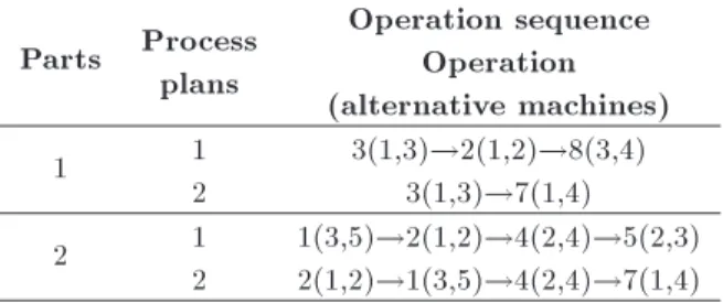
In this section, a new solution representation method is proposed to solve the FAJSS problem using the PSO algorithm. The method consists of three linked levels, and each of them is used in one of the loops. To better understand the method, an example is shown in Table 1. This table shows the alternative process plans and machines for two independent parts. Each of these parts has two alternative process plans. Two alternative machines also are available to process each operation.
4.2.1. Solution representation for process planning loop
To represent the solution in the process planning loop, an array in the length of the number of parts is
Table 1. Alternative process plans and machines for two independent parts.
Parts Process plans
Operation sequence Operation (alternative machines)
1 1
2
3(1,3)!2(1,2)!8(3,4) 3(1,3)!7(1,4)
2 1
2
1(3,5)!2(1,2)!4(2,4)!5(2,3) 2(1,2)!1(3,5)!4(2,4)!7(1,4)
Figure 3. Solution representation for process planning loop.
considered. This array corresponds to the position vector of a given particle. Each element of this array belongs to one of the parts in the problem, and the selected process plan for each part is interpreted from the assigned value to the corresponding element in the array. Figure 3 shows an example of solution representation in the process planning loop for the problem mentioned in Table 1. The position vector corresponding to the particle shown in Figure 3 is x = (1:35; 2:11). The selected process plan for each part in this solution representation method is equal to the biggest integer number below the assigned value to the corresponding element in the position vector. Considering Figure 3, the rst and second process plans are selected for parts 1 and 2, respectively. The permitted range for each element in the position vector in this loop is [1; Npp + 1), where Npp is the number of available process plans for the corresponding part. 4.2.2. Solution representation for routing loop
In this loop, an array in the length of the total number of operations of parts is considered the position vector. It is clear that this number depends on selected process plans in the process planning loop. Each element of this array belongs to one of the operations. Figure 4 shows an example of solution representation in the routing loop for the problem mentioned in Table 1, considering the selected process plans shown in Figure 3. The position vector, which corresponds to the particle shown in this gure, is x0 = (1:24; 1:75; 2:36; 1:94; 2:19; 2:97; 1:07).
In this solution representation method, the biggest integer number below the assigned value to each element in the position vector indicates the order of selected machines for operation.
For instance, in the mentioned example above, the second machine is selected for the third operation of part 1. Considering Table 1, it means that machine 4 is selected for this operation. In this loop, the permitted range for each element in the position vector is [1 + Nm + 1), where Nm is the number of available alternative machines for corresponding operations. 4.2.3. Solution representation for scheduling loop In this loop, the solution representation is based on the selected process and routing plans in the outer loops. Figure 5 shows the selected machines for the mentioned example above.
so-Figure 4. Solution representation for routing loop.
Figure 5. Selected machines for operations of the parts.
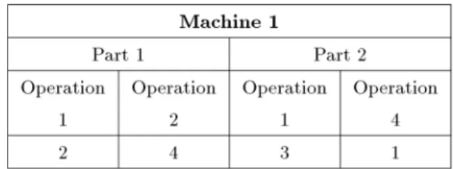
Figure 6. An example for preference list.
lution representation method in this loop. A preference list is an array, in which the order of processing on the machines is determined. The array includes some sub-arrays, each of them belonging to one of the machines. Figure 6 shows an example of machine 1 considering the information in Figure 5. As shown in Figure 6, four operations have been allocated to machine 1, which can be processed with the arrangement shown in the gure. The signicant point about the preference list is that the arrangement made for processing on the machine is not a hard rule. In other words, the operation with the topmost order in the list can be considered for processing when it's predecessors have been passed. Otherwise, the next order is considered. By this denition, all generated solutions would be feasible, which is the best characteristic of the preference list.
With regard to the specications of the preference list, after generating an arrangement, the scheduling plan can be obtained. So, the key issue in the use of this concept for a scheduling loop is how to generate all permutations of the numbers in the preference list for searching the solution space of the problem. This method also should be in accordance with the continuous nature of the PSO algorithm.
Behroozi and Eshghi [23] utilized an interesting method proposed by McCarey [24] to represent the solution of a classical job shop scheduling problem in a hybrid algorithm. McCarey [24] designed this method to generate an arbitrary permutation using a mathematical construct. This method interprets
Figure 7. Pseudo code for transformation numbers in base 10 into factoradic form.
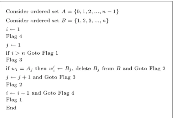
each permutation as an ordinary number in base 10 and makes a one to one mapping between them. To generate permutations in order n by this method, at rst, a number in base 10 should be transformed into factoradic form. This number could be an integer in the range of [0; n! 1]. The pseudo code of this transformation can be found in Figure 7.
In this gure, i is a counter in factoradic form from the right, and n is the order of permutations. Besides, wiindicates the ith number in factoradic form,
and h at the rst iteration is equal to the number in base 10. Moreover, bh=ic indicates the biggest integer number below h=i. We can, for example, represent 59 in factoradic form as (21210). In the factoradic form, the ith number from the right could be an integer in the range of [0; i 1]. To generate a permutation, the factoradic form should be transformed by a simple algorithm, which is shown in Figure 8. In this gure, w0 i
indicates the ith number in the permutation from the left. Also, ordered sets, A and B, mean sets in which the elements have an ascending order, based on their values. The output of this transformation would be a permutation composed by elements in set B. For better understanding, a transformation is performed for the mentioned above example and is shown in Figure 9. At rst, 59 is transformed into factoradic form by the algorithm shown in Figure 7. Afterward, the produced array is transformed into a permutation by the algorithm shown in Figure 8. For example, consider the rst number in factoradic form. This number is the 3rd number in set A. So, the 3rd number from set B
is considered the rst number in the permutation and is deleted from set B, and so on. By this algorithm, 59 is transformed into (32541) as the 59th permutation in order 5. In order to utilize this method for the solution representation in the scheduling loop, we introduce two strategies:
Strategy I: This strategy is similar to the strategy applied by Behroozi and Eshghi [23]. In this strategy, an array is considered for each machine as a preference list. The length of each array is equal to the number of operations assigned to the corresponding machine.
Figure 8. Pseudo code for transformation of factoradic form into a permutation.
Figure 10 shows the preference lists for the men-tioned example in Table 1. By this strategy, each element of the position vector belongs to a machine and could have a value in the range of [0; Nam!), where Nam is the number of assigned operations to the machine. First, in the algorithm, the biggest integer number below the value of the element in the position vector is considered. This value is transformed into factoradic form. Afterward, the factoradic form is changed to a permutation in order Nam. This permutation could be interpreted as a preference list for the machine. Figure 10 indicates an example of the solution representation for the scheduling loop by Strategy I. The position vector for this example is x00= (11:62; 1:35; 0:75).
This strategy could be applied successfully only in situations where the number of assigned operations to the machines is low. Imagine, for example, that 100 operations are assigned to a machine. Under such a condition, the element corresponding to this machine in the position vector could have a value in the range of [0; 100!). So, the algorithm may be faced with very large values.
Strategy II: The type of array in this strategy is partly similar to Strategy I. The main dierence between them is in the representation of the position vector. As mentioned before, in factoradic form, the ith number from the right could be an integer in the range
Figure 9. An example for transformation of an integer into a permutation.
Figure 11. Solution representation for scheduling loop by Strategy II.
of [0; i 1]. This characteristic is used in this strategy to specify the position vector. On this basis, each element of a given preference list has a corresponding element in the position vector. This element in the position vector can have a real value in the range of [0; i). In addition, the biggest integer number below this value is considered in factoradic form. After the formation of the factoradic form, like Strategy I, it is transformed into a permutation and a preference list is made. Figure 11 explains this process. By this strategy, the position vector for the above example is x00 = (1:25; 2:13; 1:76; 0:43; 1:01; 0:54; 0:71). The
biggest integer number below these values is considered as the factoradic form and is used to generate the preference list. Therefore, for the above example, the preference list would be the same as shown in Figure 10. Using strategy II, the algorithm no longer needs to use the number in base 10 and is not faced with large values. So, this strategy is used for the solution representation in the scheduling loop.
4.3. Termination criteria
If the number of iterations in each loop reaches a pre-scribed maximum value, the loop is interrupted. The algorithm in each loop is also stopped after executing a specied number of iterations without improvement in the objective function.
5. Numerical experiment
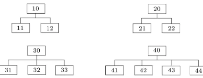
This section describes the computational tests used to evaluate the eectiveness and eciency of the proposed algorithm in nding high quality solutions. For this purpose, we tested the algorithm using some test prob-lems. The data for the problems were obtained from the part manufacturing industry. In these problems, a workshop with 6 machines is considered, whose machine 6 serves as an assembly station. Also, there are 10 types of distinct operation, where operation 6 is the assembly operation. The problems are divided into three groups; small, medium and large size problems. Each group, based on the number of available process plans and alternative machines, is also divided into 4 problems. In the problems, 4 jobs with 15 parts are considered. Predecessor/successor relationships between these parts are shown in Figure 12. In the small size problems, jobs 1 and 2 are considered;
Figure 12. Predecessor/successor relationships for all parts in the test problems.
therefore, these problems contain 6 parts. The medium size problems include jobs 1, 2 and 3; consequently, there are 10 parts in these problems. Finally, the large size problems consider all jobs with 15 parts. Also, there are some identical parts in the problems; parts 11, 12 and 21 are similar to parts 31, 22 and 41, respectively, which are labeled distinctly.
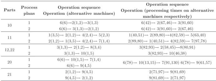
The number of operations for the parts varies between 2 to 4. Tables 2 and 3 show the details of one of the test problems. As seen in Table 3, the setup times between identical parts have been considered to be zero. Also, \Dummy" in this table indicates the dummy job mentioned in Section 2.
To solve these problems, we coded the mathemat-ical model proposed by Nourali et al. [18] by GAMS software, which solved them by the branch and bound method. The running time for solving problems by the software was limited to 3600 seconds. We also coded the proposed algorithm by C++ language. This program, and GAMS software was run on a laptop with a 2.4 GHz Intel Core i3 processor and 4 GB RAM. Based on some preliminary experiments, the following parameters were applied to the proposed algorithm: The swarm size for each loop is 10. The value of 2 has been considered for both learning factors, c1
and c2. The maximum number of iterations in the
process planning, routing and scheduling loops is 10, 20 and 30, respectively. The maximum number of iterations, without improvement in objective function for each loop, is equal to half the maximum number of iterations. For all the loops, inertia weight is adjusted via the following relation:
w = wmax wmaxN wmin PSO t;
Table 2. Details of problem P1-1. Parts Process
plans
Operation sequence Operation (alternative machines)
Operation sequence
Operation (processing times on alternative machines respectively)
10 1
2
6(6)!2(1,2)!3(1,3) 6(6)! 3(1,3)!2(1,2)
6(42)! 2(67,46)! 3(91,60) 6(42)! 3(91,60)! 2(67,46)
11 1
2
1(3,5)! 2(1,2)! 4(2,4)! 5(2,3) 2(1,2)! 1(3,5)! 4(2,4)! 7(1,4)
1(40,51)! 2(89,80)!4(82,59)! 5(63,40) 2(89,80)! 1(40,51)! 4(82,59)! 7(97,78)
12,22 1
2
3(1,3)! 2(1,2)! 8(3,4) 3(1,3)! 10(1,5)
3(82,93)! 2(58,45)!8(80,91) 3(82,93)! 10(46,38)
20 1
2
6(6)! 10(1,5)! 7(1,4)
6(6)! 9(4,5) 6(78)! 10(13,15)! 7(91,130) 6(78)! 9(61,57)
21 1
2
2(1,2)! 9(4,5) 9(4,5)! 2(1,2)
2(71,97)! 9(81,69) 9(81,69)! 2(71,97) Table 3. Sequence dependent setup times for problem
P1-1.
Machines From parts To parts 10 11 12 20 21 22
1 Dummy 29 28 24 14 24 27
10 - 14 22 16 15 18
11 29 - 16 23 16 16
12 25 25 - 28 16 0
20 26 19 25 - 19 19
21 14 23 27 21 - 26
22 25 25 0 28 16
-2 Dummy 30 19 29 - 23 19
10 - 16 17 - 19 10
11 12 - 21 - 17 24
12 14 17 - - 23 0
20 - - -
-21 25 18 29 - - 18
22 14 17 0 23
-3 Dummy 24 27 18 - - 28
10 - 24 16 - - 24
11 14 -20 - - 14 0
12 26 26 - - - 0
20 - - -
-21 - - -
-22 26 26 0 - -
-4 Dummy - 16 17 27 23 15
10 - - -
-11 - - 18 21 16 19
12 - 17 - 19 27 0
20 - 21 12 - 15 30
21 - 15 19 12 - 27
22 - 17 0 19 27
-5 Dummy - 22 30 16 17 30
10 - - -
-11 - - 24 27 19 27
12 - 21 - 23 19 0
20 - 26 19 - 26 19
21 - 30 24 29 - 24
22 - 21 0 23 19
-6 Dummy 26 - - 30 -
-10 - - - 26 -
-11 - - -
-12 - - -
-20 30 - - - -
-21 - - -
-22 - - -
-Figure 13. Gantt chart for problem P1-1.
for inertia weight and are set as 1 and 0.5, respectively. NPSO is also the maximum number of iterations for
each loop. Due to the non-deterministic nature of the algorithm, the solutions for each problem have been obtained with 10 replications. Figure 13 illustrates a Gantt chart of the solution obtained for the test problem P1-1. In this gure, the operations have been shown by white rectangles and labeled via ijl, which means the lth operation of part ij and the black rectangles show setups.
The results for all test problems are shown in Table 4. With respect to the obtained results, the following comments can be made:
The branch and bound method could nd optimal solutions for small size problems. Therefore, the results of these problems can be considered a good benchmark for the proposed algorithm.
The branch and bound method failed to nd the rst mixed integer programming solution for one of the large size problems in determined time limitation.
bound method and the proposed algorithm in small size problems shows that the algorithm could nd the optimal solution in three of them in an ideal time.
The investigation of the results obtained by the branch and bound method in the small size problems shows that the time of solving by this method is strongly sensitive to exibility levels, while the proposed algorithm shows much less time sensitivity to exibility levels in nding the optimal solution for these problems.
The obtained results from the proposed algorithm in medium and large size problems are considerable compared with the results of the branch and bound method. In these problems, the best solutions obtained by the proposed algorithm have a signif-icant dierence compared to the best mixed integer programming solutions obtained by the branch and bound method. In some cases, this dierence is even seen between the average of solutions found by the algorithm and the best mixed integer pro-gramming solutions obtained by the branch and bound method. Moreover, the algorithm has found these solutions in much less time than the branch and bound method, which indicates the merit of the proposed algorithm in solving large size prob-lems.
6. Conclusions
This paper has proposed a PSO-based optimization approach to handle a FAJSS problem with sequence dependent setup times, with the objective of minimiza-tion of makespan. The algorithm includes three nested loops, which use a new solution representation to solve the problem. The eectiveness and eciency of the algorithm has been validated by comparing the branch and bound method on some application instances. Whereas the parameters of the proposed algorithm have been adjusted based on limited experiments, the use of a structured technique is recommended. Besides, considering the assumptions, such as operation costs and resource capacity, the development of new methods for solution representation may be considered for future research.
Abbreviations
IPPS Integration of Process Planning and Scheduling
NLPP Non-Linear Process Planning PSO Particle Swarm Optimization
FAJSS Flexible Assembly Job Shop Scheduling
References
1. Benjaafar, S. and Ramakrishnan, R. \Modelling, mea-surement and evaluation of sequence exibility in manufacturing systems", Int. J. of Prod. Res., 34(5), pp. 1195-1230 (1996).
2. Tan, W. and Khoshnevis, B. \Integration of process planning and scheduling - A review", J. of Intell. Manuf., 11, pp. 51-63 (2000).
3. Jain, A. Jain, P.K. and Singh, I.P. \Integrated scheme for process planning and scheduling in FMS", Int. J. of Adv. Manuf. Technol., 30(11-12), pp. 1111-1118 (2006).
4. Anosike, A.I. and Zhang, D.Z. \An agent-based ap-proach for integrating manufacturing operations", Int. J. of Prod. Econ., 121(2), pp. 333-352 (2009). 5. Kempenaers, J., Pinte, J., Detand, J. and Kruth,
J.P. \A collaborative process planning and scheduling system", Adv. in Eng. Softw., 25(1), pp. 3-8 (1996). 6. Li, X., Shao, X., Gao, L. and Qian, W. \An eective
hybrid algorithm for integrated process planning and scheduling", Int. J. of Prod. Econ., 126(2), pp. 289-298 (2010).
7. Tan, W. and Khoshnevis, B. \A linearized polynomial mixed integer programming model for the integration of process planning and scheduling", J. of Intell. Manuf., 15(5), pp. 593-605 (2004).
8. Ozguven, C., Ozbakir, L. and Yavuz, Y. \Mathe-matical models for job-shop scheduling problems with routing and process plan exibility", Appl. Math. Model., 34(6), pp. 1539-1548 (2010).
9. Imanipour, N., Zegordi, S.H. and Osati, M. \A heuristic approach for minimizing maximum absolute lateness in exible job shop problem", Proc. of 35th Int. Conf. of Comput. and Ind. Eng., Istanbul, Turkey, 1, pp. 973-978 (2005).
10. Imanipour, N. \Modeling & solving exible job shop problem with sequence dependent setup times", Proc. of Int. Conf. on Serv. Syst. and Serv. Manag. 2, art. 4114662, pp. 1205-1210 (2006).
11. Li, W.D. and McMahon, C.A. \A simulated annealing-based optimization approach for integrated process planning and scheduling", Int. J. of Comput. Integr. Manuf., 20(1), pp. 80-95 (2007).
12. Moon, C. and Seo, Y. \Evolutionary algorithm for advanced process planning and scheduling in a multi-plant", Comput. and Ind. Eng., 48(2), pp. 311-325 (2005).
13. Moon, C., Lee, H.Y., Jeong, C.S. and Yun, Y. \In-tegrated process planning and scheduling in a supply chain", Comput. and Ind. Eng., 54(4), pp. 1048-1061 (2008).
14. Guo, Y.W., Li, W.D., Mileham, A.R. and Owen, G.W. \Applications of particle swarm optimisation in
inte-grated process planning and scheduling", Robot. and Comput. Integr. Manuf., 25(2), pp. 280-288 (2009). 15. Shao, X., Li, X., Gao, L. and Zhang, C. \Integration
of process planning and scheduling-A modied genetic algorithm-based approach", Comput. and Oper. Res., 36(6), pp. 2082-2096 (2009).
16. Li, X., Gao, L., Shao, X., Zhang, C. and Wang, C. \Mathematical modeling and evolutionary algorithm-based approach for integrated process planning and scheduling", Comput. and Oper. Res., 37(4), pp. 656-667 (2010).
17. Wang, Y.F., Zhang, Y.F. and Fuh, J.Y.H. \A PSO-based multi-objective optimization approach to the Integration of process planning and scheduling", 8th IEEE Int. Conf. on Control. and Autom., Xianmen, China, art. 5524365, pp. 614-619 (2010).
18. Nourali, S., Imanipour, N. and Shahriari, M.R. \A mathematical model for integrated process planning and scheduling in exible assembly job shop environ-ment with sequence dependent setup times", Int. J. of Math. Anal., 6(43), pp. 2117-2132 (2012).
19. Mckoy, D.C. and Egbelu, P.J. \Minimizing production ow time in a process and assembly job shop", Int. J. of Prod. Res., 36(8), pp. 2315-2332 (1998).
20. Kennedy, J. and Eberhart, R.C. \Particle swarm optimization", In Proc. of IEEE Int. Conf. on Neural Netw., New Jersey, IEEE Service Center, pp. 1942-1948 (1995).
21. Poli, R., Kennedy, J. and Blackwell, T. \Particle swarm optimization: An overview", Swarm Intell. 1, pp. 33-57 (2007).
22. Lei, D. \A pareto archive particle swarm optimization
for multi-objective job shop scheduling", Comput. and Ind. Eng., 54, pp. 960-971 (2008).
23. Behroozi, K. and Eshghi, M. \A new hybrid particle swarm optimization for job shop scheduling problem", Int. J. of Ind. Eng. and Prod. Res., 20(2), pp. 57-75 (2009).
24. McCarey, J. \Using permutations in. NET for im-proved systems security", Volt Inf. Sci. (2003).
Biographies
Saeid Nourali obtaned a BS degree in Industrial En-gineering from Shomal University, Mazandaran, Iran, and his MS degree in Industrial Management from the Faculty of Management and Accounting at Islamic Azad University, South Tehran Branch, Iran, in 2011. His main research interests include production planning and scheduling, meta-heuristics, project management and decision Theory. He has also published journal papers in the elds of operation management and decision sciences.
Narges Imanipour obtained a BS degree in Indus-trial Engineering from Sharif University, Tehran, Iran, and MS and PhD degrees in Industrial Engineering from Tarbiat Modares University, Tehran, Iran. She is currently Associate Professor of the Faculty of Entrepreneurship at the University of Tehran, Iran. Her primary areas of interests are production plan-ning and scheduling, meta-heuristics, decision making, new venture creation and small-medium sized enter-prises.