A Heuristic Algorithm and a Lower Bound
for the Two-Echelon Location-Routing
Problem with Soft Time Window Constraints
E. Nikbakhsh
1and S.H. Zegordi
1;Abstract. The location-routing problem is one of the most important location problems for designing integrated logistics systems. In the last three decades, various types of objective function and constraints have been considered for this problem. However, time window constraints have received little attention, despite their numerous real-life applications. In this article, a new 4-index mathematical model, an ecient and fast heuristic and a lower bound for the two-echelon location-routing problems with soft time window constraints are presented. The proposed heuristic tries to solve the problem via creating an initial solution, then improving it by searching on six neighborhoods of the solution, and using the Or-opt heuristic. At the end, computational results show the eciency of the proposed heuristic, using the proposed lower bound.
Keywords: Location-routing; Location; Routing; Soft time window; Heuristic algorithm.
INTRODUCTION
Integration of supply chain management activities is an important step toward the success of a supply chain. One of the main types of supply chain inte-gration involves integrating the physical material ow between suppliers, manufacturers, distribution centers and customers [1]. During the last three decades, this type of integration, known as an integrated lo-gistics system, has become one of the most important aspects of logistics and supply chain management. This concept considers the interdependence between facility location, transportation and routing structures, inventory control systems and production planning and scheduling systems for various parts of the supply chain. This comprehensive approach and simultaneous solving of logistics problems prevents the local opti-mization of dependent problems. Integrated logistics problems include dierent problems, such as location-routing [2], inventory-location [3], queuing-location [4] and inventory-routing [5] problems.
The Location-Routing Problem (LRP) tries to
1. Department of Industrial Engineering, Faculty of Engineer-ing, Tarbiat Modares University, Tehran, P.O. Box 14117-13116, Iran.
*. Corresponding author. E-mail: [email protected] Received 4September 2008; received in revised form 27July 2009; accepted 29 September 2009
jointly solve the problem of nding the optimal num-ber, the capacity, the location of facilities serving more than one supplier/customer and optimal routing struc-ture and scheduling [6]. Applications of LRPs range from bill delivery, postal system, dairy distribution and communication network designs to waste/hazardous material collection. Two main subproblems of LRP are the Location-Allocation Problem (LAP) and the Vehicle Routing Problem (VRP). Since both of these problems are NP-Hard [7,8], LRP may be considered NP-Hard as well.
The rst steps of creating LRPs dates back to the 1960s [9,10]. However, the created models were not the same as LRP, since they did not consider the trip from the last customer of the route back to the starting facility. The rst real LRP models were developed in the late 1970s and early 1980s through the eorts of various researchers [11-15].
Despite extensive applications of time window constraints in the more realistic modeling of LRP, researchers have paid little attention to LRPs with time window constraints beginning only in the early 1980s. Jacobsen and Madsen solved a one-echelon LRP with hard time windows (LRPTW) for a news-paper distribution network, using a combination of a location-allocation-rst, route-second heuristic with a tree-tour method [11] and a saving method [12]. In a two-echelon LRP model for rubber collection,
Nambiar et al. [14] considered the maximum allowed time for delivering commodities as the time window for the depots. In recent years, two researchers have considered the application of multi-echelon LRPTW in military theater distribution. Cox [16] considered the possibility of multiple trips for each and solved a mixed integer programming model using CPLEX. In addition, Burks [17] solved multi-echelon LRPTW with pick-up and delivery using a tabu search algorithm.
In recent years, researchers have considered other types of LRP. Lin et al. [18] solved a two-echelon LRP with a capacitated vehicle eet, using a three-phase heuristic based on simulated annealing, branch and bound and the traveling salesman problem. Wu et al. [19] considered a one-echelon LRP with a capaci-tated heterogeneous vehicle eet, and solved it with a hybrid heuristic based on decomposition and a simu-lated annealing algorithm. Chan et al. [20] considered a LRP with a maximum route duration constraint and solved it via a saving/insertion heuristic. In addition, they presented an upper and lower bound for the number of facilities and the vehicle eet size in each facility. Albareda-Sambola et al. [21] modeled a one-echelon LRP and presented an upper bound, using a tabu search and a lower bound using a saving/insertion heuristic.
More recently, Alumur and Kara [22] modeled a two-echelon LRP for hazardous material with multiple objectives as a mixed integer programming problem, and solved it via CPLEX. Ozyurt and Asken [23] presented a branch and bound scheme based on a tabu search heuristic, Lagrangian relaxation and a minimum spanning forest problem. Albareda-Sambola et al. [24] considered a LRP with stochastic customers and applied it, using a neighborhood search heuristic and a lower bound, based on decomposition of the objective function to location and m-TSP subproblems. Schwardt and Fischer [25] proposed a neural network algorithm, based on self-organizing maps for a single facility LRP in the continuous space. Finally, Am-brosino et al. [26] proposed a two-phase heuristic with a large neighborhood search, based on path and cyclic exchanges of customers among routes, for the single facility LRP.
The main reason for neglecting time window con-straints in LRP literature can be attributed to dierent planning levels and horizons of location and routing decisions; strategic and tactical, respectively. However, researchers have shown that initial simultaneous and joint decision making for these two problems leads to lower costs in the long run, even though the routes change in the course of time [27,28]. Hence, one can conclude intuitively that in the long run solving LRPTW can also lead to lower costs
The main purpose of this article is to model and solve a two-echelon location-routing problem with
soft time window constraints (2ELRPSTW). In this problem, serving each customer is possible in two consecutive time intervals. The second interval diers from the rst in the fact that serving the customer is only possible via paying a xed penalty cost. In addition, the vehicle eet capacity for each regional distribution center is considered limited. Due to working regulations and/or the requirements of the commodity being delivered, it is assumed that each vehicle can only be used for a limited duration in each working day.
For this problem, a new 4-index mathematical model and a heuristic algorithm method are presented. The proposed heuristic algorithm method is based on location-rst, allocation-routing second, for an initial solution construction and a neighborhood search and Or-opt heuristic for solution improvement. Then, a lower bound for 2ELRPTW based on objective func-tion decomposifunc-tion is presented. For the computafunc-tion of lower bound routing subproblems, existing methods for using the minimum spanning forest problem are improved via a binary programming problem. The eciency of the proposed heuristic is shown via com-putational results. Finally, research results and future research opportunities are discussed.
MATHEMATICAL MODEL
The 2ELRPSTW logistic system is dened on an undirected graph, G = (N; E). The nodes of this graph (N) consist of Central Depot Centers (CDC), Regional Depot Centers (RDC) and Customers (C). The undirected edges of this graph (E) are composed, of edges linking CDCs to RDCs, RDCs to customers and customers to customers. Triangle inequality is assumed to be valid for edges linking RDC to customers and customers to customers. It is assumed that the capacities of the CDCs, RDCs and the homogeneous vehicle eet are deterministic and known parameters. The vehicle eets assigned to RDCs are assumed homo-geneous. Finally, customer demand is also known and deterministic and cannot be split. The 2ELRPSTW parameters are as follows:
I: set of central depot center nodes, J: set of regional depot center nodes, C: set of customer nodes,
N1j: set of all nodes belonging to the set, C [ j;
8j 2 J F0
i: capacity of the ith CDC,
F Cj: xed cost of opening jth RDC,
V Cj: variable cost of operating the jth RDC for a
unit of the commodity,
CRij: cost of transportation for a unit of the
comm-odity between the ith CDC and the jth RDC, Fj: capacity of the jth RDC,
CV : xed cost of a vehicle, : vehicle capacity,
nj: maximum number of vehicles assignable
to the jth RDC (nj= dFj=e),
: maximum allowable route duration, Dk: demand of the kth customer,
tkm: travel time between the nodes k and m,
k&m 2 Nij, j 2 J,
km: travel cost between the nodes k and m,
k&m 2 Nij; j 2 J,
[ak; bk]: acceptable time interval for serving the
kth customer with no penalty,
[bk; b0k]: acceptable time interval for serving the
kth customer with penalty,
P Ck: penalty cost for serving the kth customer
in the interval [bk; b0k],
The 2ELRPSTW variables are as follows:
xij: amount of commodity to be transported
bet-ween the ith CDC and the jth RDC,
yj: binary variable for opening the jth regional
depot center,
ujl: binary variable for assigning the lth vehicle
to the jth RDC, j 2 J; l = 1; :::; nj,
kmjl : binary variable for traveling the link (k; m) by the lth vehicle of the jth RDC, k & m 2 N1j; k 6= m; j 2 J; l = 1; :::; nj,
zkj: binary variable for assigning the kth
custo-mer to the jth RDC,
wkjl: arrival time of the lth vehicle of the jth RDC to the kth customer, k 2 C; j 2 J; l = 1; :::; nj,
rjl
k: binary variable for serving the kth
custo-mer with the lth vehicle of the jth RDC in the penalized interval [bk; b0k], k 2 C; j 2 J;
l = 1; :::; nj,
The 4-index mathematical model for the 2ELRPSTW based on models proposed by Daskin [29] and Daskin et al. [30] is as follows:
min X
j2J
F Cjyj+
X
i2I
X
j2J
CRijxij
+X
j2J
V Cj
X
k2C
Dkzkj+ CV
X
j2J nj
X
l=1
ujl
+X
j2J nj
X
l=1
X
m2N1j
X
k2N1j
kmkmjl
+X
k2C
P Ck
X
j2J nvj
X
k=1
rjlk: (1)
Subject to:
X
j2J
xij Fi0 8i 2 I; (2)
X
i2I
xij Fjyj 8j 2 J; (3)
X
k2C
Dkzkj
X
i2I
xij< 0 8j 2 J; (4)
X
j2J nj
X
l=1
X
m2N1j
jlkm= 1 8k 2 C; (5)
X
k2C
Dk
X
m2N1j
jl
km 8j 2 J; l =; 1; :::; nj; (6)
X
m2N1j
kmjl X
m2N1j
mkjl = 0
8j 2 J; l = 1; :::; nj; 8k 2 N1j; (7)
X
m2N1j
mkjl + X
h2N1j
jhjl zkj 1
8k 2 C; 8j 2 J; l = 1; :::; nj; (8)
X
k2C
kjjl = ujl 8j 2 J; l = 1; :::; nj; (9)
X
k2C
jkjl = ujl 8j 2 J; l = 1; :::; nj; (10)
wjl
m wkjl+ tkm M(1 kmjl )
8k & m 2 C; 8j 2 J; l = 1; :::; nj; (11)
max ftjm; amg wjlm min f( tmj); b0mg
8m 2 C; 8j 2 J; l = 1; :::; nj; (12)
wkjl bk+ Mrjlk
8k 2 C; 8j 2 J; 8l = 1; :::; nj; (13)
wkjl> bk M(1 rkjl)
8k 2 C; 8j 2 J; 8l = 1; :::; nj; (14)
xij 0 8i 2 I; 8j 2 J; (15)
ujl 2 f0; 1g 8j 2 J; l = 1; :::; nj; (17)
kmjl 2 f0; 1g
8j 2 J; l = 1; :::; nj; 8k & m 2 N1j; (18)
zkj2 f0; 1g 8k 2 C; 8j 2 J; (19)
rjlk 2 f0; 1g 8k 2 C; 8j 2 J; l = 1; :::; nj: (20)
In the above model, Objective Function 1 includes RDCs opening xed costs, CDCs to RDCs commodity transportation costs, RDCs variable costs, vehicle eet acquisition costs, routing costs and soft time win-dows violation penalty costs. Constraint 2 limits the outgoing commodity from each CDC to its capacity, while Constraint 3 limits the incoming commodity into each RDC to its capacity. Constraint 4 balances the incoming and outgoing commodity volume at each RDC. Constraint 5 requires each customer to be on just one route belonging to one vehicle of one of the RDCs. Constraint 6 imposes a capacity restriction on each vehicle.
Constraint 7 ensures the ow conservation. Con-straint 8 assigns a customer to a RDC, if a vehi-cle from that RDC enters that customer node and leaves the RDC node itself at the beginning of its trip. Constraints 9 and 10 ensure that if a vehicle is assigned to a RDC, it both enters and leaves that RDC. Constraint 11 calculates the arrival time of vehicles to customers and also eliminates subtours [31]. Constraint 12, a generalization of Kontoravdis and Bard's model for a time window constraint [32], denes the soft time window domain for each customer. Its lower bound tightens the time window lower bound with the earliest direct arrival time of a vehicle to a customer from the origin RDC, if possible. In addition, its upper bound tightens the time window upper bound with the route maximum allowed travel time, if possible.
Constraints 13 and 14 determine if a vehicle has passed the maximum allowed time for arrival to a customer without paying a penalty (bk). Finally,
Con-straints 15 to 20 dene the variables types. The com-plexity of the above mixed integer programming model is due to the existence of soft time window constraints and the NP-Hard nature of the problem. Hence, solving medium and large-sized instances of this problem via exact methods is a challenging and dicult task.
The proposed mathematical model for the 2EL-RPSTW is based on 4-index routing variables (source node, destination node, source RDC and the vehicle number belonging to the RDC) for on routing RDC-to-customer and customer-RDC-to-customer edges. Since this 4-index model considers as many variables for each RDC as the maximum number of vehicles assignable
to that RDC, this model has fewer variables used in each constraint compared to common 3-index mod-els [29,30]. In addition, this model allows for merg-ing maximum route duration constraints with time window constraints, which has been described previ-ously.
HEURISTIC ALGORITHM
In this section, a two-phase heuristic algorithm based on the neighborhood search proposed by Albareda-Sambola et al. [24] and Or-opt heuristic [33], is pre-sented (Figure 1). In the construction phase, an initial solution is created with a location-rst, allocation-routing-second algorithm and then improved with an Or-opt heuristic. Then, in the improvement phase, the nal solution is obtained by searching six neigh-borhoods of the initial solution and Or-opt heuristic. Construction Phase
1. Location: In this step, RDCs to be opened are found sequentially based on the ratio of their xed cost to their capacity. An unopened RDC with a minimum ratio is selected for allocating customers to it.
2. Allocation-Routing: In this step, customers
are added to the last opened RDC and inserted into routes using the modied Balakrishnan algo-rithm [34], based on the minimum weighted sum of the routing time, amount of soft time window violation and customer priority. In each customer allocation, none of the Constraints, 3, 6 and 12 can be violated. If all customers are not allocated to the current opened RDCs, the location step will be repeated until all customers are allocated to the opened facilities. In this step, the maxi-mum allowed soft time window constraints violation penalty cost is restricted to 20% of its total sum. 3. Initial Route Improvement: In this step, the
initial routes of step 2 are improved via the Or-opt heuristic.
Improvement Phase
In this phase, the initial solution derived from phase one is improved by searching on six neighborhoods of the initial solution. In addition, the Or-opt heuristic is used to improve each route with intra-route exchanges. All moves are performed with respect to the amount of total saving due to changes in the RDCs xed cost, RDCs variable costs, transportation between CDCs and RDCs, routing costs and soft time windows violation penalty costs. Also, in this phase, the same feasibility conditions as the feasibility conditions of step 2 of phase one are controlled.
Six neighborhoods of the improvement phase are an extension of the algorithm proposed by Albareda-Sambola et al. [24] for the single-echelon LRP. Albareda-Sambola et al. [24] proposed four neighbor-hoods (N1(x); N2(x); N3(x) and N4(x)) for a local
search in a LRP with a stochastic customer presence. The new neighborhood N5(x) exchanges the starting
RDC of two routes. In each solution belonging to N5(x), the starting RDCs of two routes belonging to
ith RDC and jth RDC are set to jth RDC and ith RDC, respectively. In addition, the new neighborhood N6(x) adds a new route to a RDC with the least used
capacity ratio, and then, some customers from other routes are removed and inserted into the new route. A search on the four neighborhoods of step 2.1 of Figure 1 improves the current solution with respect to current opened RDCs. In addition, two neighborhoods of steps 2.3 and 2.4 of Figure 1 diversify the search space with opening new RDCs.
Stopping Criteria
If no feasible move is performed while searching neigh-borhoods N3(x) and N4(x), then the algorithm stops.
In addition, if the amount of saving between two main algorithm iterations is less than a specied value, ", then the algorithm stops.
LOWER BOUND COMPUTATION
For computing the lower bound of the objective func-tion of Problem (1-20), ZLB, the set of constraints
linking the location and routing subproblems (Con-straint 8) are relaxed and the customers-to-RDCs assignment variables are omitted. Then, each of the location (Z1) and routing (Z2) subproblems are
minimized, regarding their respective constraints. The rst subproblem consists of the xed and variable costs of RDCs and the costs of CDCs to RDCs commodity transportation. The second subproblem consists of the vehicle acquisition xed costs, routing costs and soft time windows violation penalty costs. The rst sub-problem is a location sub-problem. The second subsub-problem can be converted to a degree-constrained capacitated Minimum Spanning Forest Problem (MSFP) with max-imum route duration, after the necessary modications. Lower Bound Location Subproblem
Before obtaining the rst subproblem solution, imple-mentation of the following modication is necessary. Since the Minimum Spanning Forest Problem (MSFP) neglects the cost of returning from the last customer in each route to the RDC, the term min
m2Cfmjg:nj:src
is added to the xed cost of each RDC, F Cj, as
an estimate of the return cost to the RDC. In the aforementioned term, src is used to compensate for
the possible overestimation caused by nj, and it
is calculated as the average of the ratio of vehicles assigned to each opened RDC to the maximum number of vehicles assignable to that RDC in the nal solution of the proposed heuristic for each test problem size. The objective function and constraints of the lower bound location subproblem are as follows:
min Z1=
X
j2J
F Cjyj+
X
i2I
X
j2J
CRijxij
+X
j2J
V Cj
X
i2I
xij; (21)
Subject to: X
j2J
xij Fi0 8i 2 I; (22)
X
i2I
xij Fjyj 8j 2 J; (23)
X
i2I
X
j2J
xij =
X
k2C
Dk: (24)
In the above problem, Constraints 22 and 23 are the same as Constraints 2 and 3. Constraint 24 makes the total amount of the commodity transported from CDCs to RDCs equal the total demand.
Lower Bound Routing Subproblem
The application of MSFP with the degree, vehicle capacity and route duration constraints, in solving the LRP and obtaining its solution, using Prim's algorithm [35], has received little attention from re-searchers [23,36]. This problem in its simplest case (relaxing vehicle capacity and route duration con-straints) on a connected graph is a degree-constrained minimum spanning tree problem that is known to be NP-Complete [37]. Hence, obtaining its optimal solution in polynomial time using exact optimization techniques is not possible. The objective function of the second subproblem of Objective Function 1, after relaxing soft time window constraints, is as follows:
Z2= CV
X
j2J nj
X
l=1
ujl+
X j2J nj X l=1 X m2N1j X k2C
mkmkjl :
(25) For transforming Objective Function 25 into a degree-constrained capacitated MSFP with route duration constraints, the vehicle acquisition xed cost term must be omitted via adding the vehicle xed cost to all of the edges emerging directly from RDCs to customers. This modication also restricts the irregular emerging edges from the RDCs selection and hence, an unrealistic customer service scheme. Then, the remaining con-straints must be modied so that a degree-constrained capacitated MSFP with route duration constraints is obtained. The objective function and constraints of this problem are as follows:
min Z0
2= X j2J nj X l=1 X k2C
(jk+ CV )jkjl
+X j2J nj X l=1 X m2C X k2C
mkmkjl : (26)
Subject to: X j2J nj X l=1 X m2N1j
mkjl = 1 8k 2 C; (27)
X k2V X m2V X j2J nj X l=1 nj
km jV j 1
2 jV j jCj; 8V C; (28)
X j2J nj X l=1 X m2C
jmjl +X
j2J nj X l=1 X k2C X m2C m>k
jlkm= jCj; (29) X j2J nj X l=1 X m2C jmjl & X k2C
Dk=
' ; (30) nj X l=1 X m2C
jmjl nj 8j 2 J; (31)
X j2J nj X l=1 X m2C jl
km 1 8k 2 C; (32)
X
m2N1j
X
k2C
tmkmkjl 8j 2 J; l = 1; :::; nj; (33)
X
k2C
Dk
X
m2N1j
mkjl 8j 2 J; l = 1; :::; nj: (34)
In the above problem, Constraint 29 sets total number of selected edges to the number of customers. Con-straint 30 guarantees the selection of at least as many edges as the minimum required number of vehicles to emerge from RDCs. Constraint 31 limits the number of outgoing edges at each RDC node to the maximum number of vehicles allowed to assign to that RDC. Constraint 32 limits the maximum number of outgoing edges at each customer node to one. The remaining constraints are the same as the similar constraints of Problem (1-20).
Since regular algorithms for the MSFP such as Prim and Kruskal [38], cannot consider maximum route duration and vehicle capacity constraints, Constraints 33 and 34 are relaxed using Lagrangian relaxation [39]. Hence, the right-hand side of these constraints is subtracted from their left-hand side, and then, the dierence is multiplied with nonnegative Lagrangian multipliers, and . Finally, these terms are added to the objective function to create the new Lagrangian function, Z0
2(; ).
Z0
2(; ) =
X j2J nj X l=1 X k2C
(jk+ CV )jkjl
+X j2J nj X l=1 X m2C X k2C
mkmkjl
+X j2J nj X l=1 jl 0 @ X m2N1j X k2C
Dkmkjl
1 A +X j2J nj X l=1 jl 0 @ X m2N1j X k2C
tmkmkjl
1 A :
(35) It is known that the maximum of the minimum of the Lagrangian Function 35 (Z0
2 (; )) regarding
and , subject to Constraints 27 to 32, is a lower bound for Objective Function 25 [40]. For solving this maximization problem, a subgradient search method (Figure 2) [41] is used for nding the Lagrangian
Figure 2. Lagrangian multipliers search algorithm.
multipliers maximizing objective function, Z0
2(; ). In
addition, an extended Kruskal algorithm (Figure 3) is used for solving Z0
2(; ). In each of the subgradient
search method iterations, a step is taken along the Lagrangian function subgradient, regarding the La-grangian multipliers values. Let the LaLa-grangian mul-tipliers vector of Lagrangian Function 35, consisting of and , be shown by vector and matrix A be the technology matrix of two Lagrangian-relaxed constraints. Also, let be the right-hand side vector of these constraints. Lagrangian multipliers values and a Lagrangian multiplier step-size modier are updated using the following equations:
(k+1)= maxf0; (k)+ t
k:(AV(k) )g; (36)
tk = u(Z
0
2 (; ) Z
0(k)
2 ((k); (k)))
jjAV(k) jj2 : (37)
In Equation 37, Z0
2 (; ), the upper bound of
La-grangian Function 35, is estimated using the routing objective function of the proposed heuristic. The Lagrangian multiplier step-size modier, u, in Equa-tion 37 is used for correcting the error of overshooting the Z0
2 (; ) upper bound.
The initial edge nding Problem (38-42), in step 2 of the extended Kruskal algorithm (Figure 3), tries to minimize the total weight of the selected edges. Con-straint 39 results in selecting exactly the same number of edges as the minimum number of required vehicles. Constraint 40 limits the number of derived edges from each RDC to the maximum number of vehicles allowed to assign to that RDC. Constraint 41 assigns each customer to at most one RDC. Finally, Constraint 42
Figure 3. Extended Kruskal algorithm.
denes the assignment variable of the kth customer to the jth RDC as a binary variable. The solution of this problem is an improvement on the methods available in the literature [23,36], resulting in better solutions by not eliminating shorter edges because of node degree constraints. This binary programming problem can be solved optimally by means of common optimization software.
For adapting Lagrangian Function 35 to the stan-dard Kruskal algorithm objective function, the 3rd and 4th terms of this function are integrated with the cost coecient of the 1st and 2nd terms, as in Equation 43.
Z0
2(; ) =
X
j2J nj
X
l=1
X
k2C
(jk+ CV + jl:Dk
+ jl:tjk)jkjl +
X
j2J nj
X
l=1
X
m2C
X
k2C
(mk
+ jl:Dk+ jl:tmk)mkjl
X
j2J nj
X
l=1
(jl + jlj): (43)
Validation of the Lower Bound ZLB
In the last two previous subsections, the minimum values of location subproblem, Z
1, and routing, Z2 =
Z0
2(; ), were derived using an exact algorithm and a
ZLB = Z1+ Z2 is a valid lower bound for Objective
Function 1 using the following axiom and lemma. Axiom
Function H(X; Y ) is composed of two functions, H1(X)
and H2(Y ). The minimum value of H(X; Y ) is greater
than/equal to the summation of H1(X) and H2(Y )
minimum values. Lemma
ZLB is a valid lower bound for Objective Function 1.
Proof
Objective Function 1 is composed of two subproblems, Z1and Z2. Solving Objective Function 21, with respect
to Constraints 22 to 24, minimizes subproblem Z1
optimally. Also, the maximum value of the mini-mization problem, consisting of Objective Function 35, with respect to Constraints 27-32 is a lower bound for subproblem Z2. Hence, according to the stated axiom,
ZLB = Z1+ Z2 is a valid lower bound for Objective
Function 1.
COMPUTATIONAL RESULTS
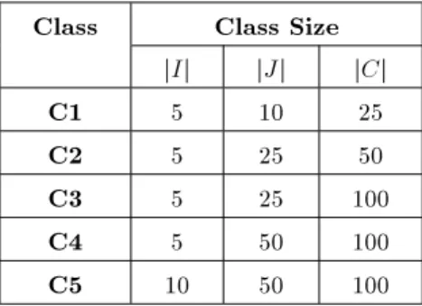
Test Problems and Algorithms Implementation For evaluation of the eciency of the proposed heuris-tic, 21 random test problems are designed and used. The graph nodes are selected randomly on a 1000*1000 Euclidean space. Table 1 contains the information regarding the size of the test problems created in 5 classes. In these problems, the distribution of customer demand, RDCs and CDCs capacities are U[7; 30], U[30; 140] , and U[100; 600], respectively. Each vehicle xed cost is set to 250, RDCs xed and variable costs are set to U[20; 80] + U[100; 110]:F2
j and U[1:5; 3] +
U[0:01; 0:03]F
j, respectively.
Transportation costs between CDCs and RDCs nodes and routing cost between RDCs and customers nodes are 0.0075 and 0.5 per Euclidean distance unit, respectively. Total RDCs capacity to total demand ratios are set to be two and ve. Vehicle capacity and maximum allowed route duration are designed, such that each route has between 5 and 10 customers.
Table 1. Problem instances class size. Class Class Size
jIj jJj jCj C1 5 10 25 C2 5 25 50 C3 5 25 100 C4 5 50 100 C5 10 50 100
Finally, soft time window violation penalty costs, P Ck,
are dened by U[120; 180] + Dk:U[3; 5], and each
cus-tomer's time window is dened by Equations 44 to 48:
ck = U[0:15; 0:85]; (44)
lk = N[0:1; 0:04]; (45)
ak= maxf0; ck lkg; (46)
b0
k = minfck+ lk; g; (47)
bk = b0k lk=2: (48)
For evaluation of the proposed heuristic eciency, six small-sized test problems (class 1), six medium-sized test problems (class 2) and nine large-medium-sized test problems (classes 3, 4 and 5; each one three instances), are selected. From these 21 test problems, the small-sized ones are solved via the LINGO optimization pack-age besides the proposed heuristic for the purpose of identifying the amount of closeness of the heuristic nal solution and the lower bound to the global optimum. Based on the initial experimental results, the routing values of the proposed heuristic, src, for small, medium
and large-sized problems are set to 0.93, 0.88 and 0.81, respectively. All the proposed algorithms and classical optimization techniques are implemented using C# 2.0 and LINGO 8.0. These programs were run on a personal computer with a 2130 MHz CPU and one GB RAM.
Experiments Results
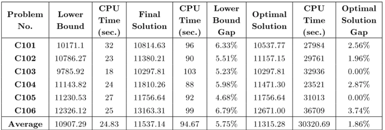
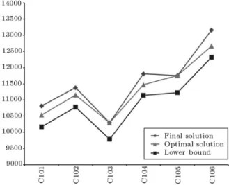
Regarding the computational results of the proposed heuristic (Tables 2 to 4), this method has an ecient and fast performance. The average lower bound gap for small, medium and large-sized test problems is 5.75%, 8.68% and 11.22%, respectively. The reason for the decline in the performance of the proposed heuristic along with the increase in the number of customers in the test problems from 25 to 100 (Figures 4 and 5) can be attributed to the growth of the solution space of the neighborhood search phase and the local search nature of the proposed heuristic. Also, the absence of considering soft time windows in the proposed lower bound can lead to an increase in this gap between the nal solution and the lower bound. However, this eect is reduced and controlled via restricting the maximum allowed soft time window constraints violation penalty to 20% of its total sum. Also, by comparison of the proposed heuristic nal solution to the optimal solutions obtained by LINGO, there is an average of a 1.86% gap with the optimal solution. Therefore, it seems that the heuristic solution is stronger from the lower bound and closer to the global optimum.
Table 2. Computational results for small-sized problems. Problem
No.
Lower Bound
CPU Time (sec.)
Final Solution
CPU Time (sec.)
Lower Bound Gap
Optimal Solution
CPU Time (sec.)
Optimal Solution
Gap C101 10171.1 32 10814.63 96 6.33% 10537.77 27984 2.56% C102 10786.27 23 11380.21 90 5.51% 11157.15 29761 1.96% C103 9785.92 18 10297.81 103 5.23% 10297.81 32936 0.00% C104 11143.82 24 11810.26 88 5.98% 11471.30 23521 2.87% C105 11230.53 27 11756.64 92 4.68% 11756.64 31013 0.00% C106 12326.12 25 13163.31 99 6.79% 12671.00 36709 3.74% Average 10907.29 24.83 11537.14 94.67 5.75% 11315.28 30320.69 1.86%
Table 3. Computational results for medium-sized problems. Problem No. Lower Bound CPU Time
(sec.) Final Solution
CPU Time (sec.)
Lower Bound Gap C201 14948.45 663 16136.99 164 7.95% C202 13223.91 613 14509.45 168 9.72% C203 14021.72 666 15182.83 178 8.28% C204 15751.13 573 17060.76 190 8.31% C205 12290.65 634 13507.04 201 9.90% C206 13837.21 574 14932.74 162 7.92% Average 14012.18 620 15221.64 177.17 8.68%
Table 4. Computational results for large-sized problems.
Problem No. Lower Bound CPU Time(sec.) Final Solution CPU Time(sec.) Bound GapLower C301 20989.41 6362 23034.85 260 9.75% C302 18190.95 6503 20380.6 286 12.04% C303 19382.03 6356 21687.43 281 11.89% C401 25270.54 6378 28209.48 277 11.63% C402 19190.39 6031 21417.79 252 11.61% C403 22835.8 6988 25067.38 265 9.77% C501 32413.05 5950 36158.71 235 11.56% C502 36821.07 6141 40598.12 269 10.26% C503 36585.15 6342 41161.64 271 12.51% Average 25742.04 6339 28635.11 266.22 11.22%
From a solution CPU time perspective, the pro-posed heuristic performs rapidly. This method solves small-sized problems in a small amount of time (av-eragely around 1.5 minute). It also solves medium and large-sized problems in a reasonable amount of time (averagely 3 and 4.5 minutes, respectively). It can be observed that CPU time has a direct relation-ship with the test problem size, and increases along with an increase in the number of customers because of the diculty of solving the classical optimization
problems. The lower bound CPU time in the largest problem instance is still less than 105 minutes, which is acceptable, considering the strategic nature of deci-sion making problems. The main factor determining the proposed lower bound CPU time is solving the location subproblem optimally, which requires more CPU time along with an increase in the number of customers.
Altogether, the proposed heuristic has an 8.55% average lower bound gap and 179.35 sec average CPU
Figure 4. Comparison of the optimal solution/heuristic solution/lower bound for small-sized problems.
Figure 5. Comparison of the heuristic solution/lower bound for medium and large-sized problems.
time, which has an acceptable lower bound gap due to the fast performance and heuristic nature of the proposed solution algorithm.
CONCLUSION
In this article, a special case of integrated logistics problems, a two-echelon location-routing problem with time window constraints, was reviewed, modeled and solved. The location-routing problem is a barrier to the local optimization of location and routing decisions because of considering the interdependence between facility location, customer assignment and the struc-ture of the routes. Despite the initial attention of re-searchers to location-routing problems with hard time window constraints, little attention has been paid to this practical problem during recent years. Therefore, the consideration of soft time window constraints is the distinguishing feature of this article.
For this problem, a new 4-index mixed integer
programming model was developed. This model has fewer variables used in each constraint compared to common 3-index models. In addition, it allows for merging maximum route duration constraints with time window constraints. Then, a two-phase heuristic, based on location-rst, allocation-routing second for initial solution construction and a neighborhood search for an initial solution improvement was developed. In addition, a lower bound for this problem was designed, based on objective function decomposition. For the routing subproblem of the lower bound, a Lagrangian relaxation scheme and the minimum spanning forest problem were used. Finally, the eciency of the proposed heuristic was shown using the proposed lower bound.
Further research opportunities include the ap-plication of metaheuristics, such as tabu search and simulated annealing, improvement of the proposed heuristic via dening new neighborhoods for local search and consideration of other local search mech-anisms, considering other types of time window vi-olation penalty functions, and nally, integration of other logistics problems, such as inventory control with LRPTW.
ACKNOWLEDGMENT
The authors would like to thank the two anonymous referees for their constructive comments and sugges-tions, which have greatly enhanced the quality of this paper.
REFERENCES
1. Hosseini Baharanchi, S.R. \Investigation of impact of supply chain integration on product innovation and quality", Scientia Iranica, Trans. E, 16(1), pp. 81-89 (2009).
2. Nagy, G. and Salhi, S. \Location-routing: issues, models and methods", European Journal of Opera-tional Research, 177(2), pp. 649-672 (2007).
3. Daskin, M.S., Coullard, C.R. and Shen, Z.-J.M. \An inventory-location problem: formulation, solu-tion algorithm and computasolu-tional results", Annals of Operations Research, 110, pp. 83-106 (2002). 4. Shavandi, H. and Mahlooji, H. \Fuzzy hierarchical
queuing models for the location set covering problem in congested systems", Scientia Iranica, 15(3), pp. 378-388 (2008).
5. Baita, F., Ukovich, W., Pesenti, R., and Favaretto, D. \Dynamic routing-and-inventory problem: a review", Transportation Research Part A, 32, pp. 585-598 (1998).
6. Min, H., Jayaraman, V. and Srivastava, R. \Com-bined location-routing problems: a research direc-tions synthesis and future", European Journal of Operational Research, 108, pp. 1-15 (1998).
7. Cordeau, J.-F., Laporte, G., Savelsbergh, M.W.P. and Vigo, D. \Vehicle routing", In Handbook of Op-erations Research and Management Science - Trans-portation, Barnhart, C. and Laporte, G., Eds., pp. 367-428, Elsevier, Amsterdam (2006).
8. Megiddo, N. and Supowit, K.J. \On the complexity of some common geometric location problems", SIAM Journal on Computing, 13, pp. 182-196 (1984). 9. Maranzana, F.E. \On the location of supply points
to minimize transport costs", Operational Research Quarterly, 15, pp. 261-270 (1964).
10. Webb, M.H.J. \Cost functions in the location of depots for multiple-delivery journeys", Operational Research Quarterly, 19(3), pp. 311-320 (1968). 11. Jacobsen, S.K. and Madsen, O.B.G. \On the location
of transfer points in a two-level newspaper delivery system - A case study", The International Symposium on Locational Decisions, Ban, Alberta, Canada (1978).
12. Jacobsen, S.K. and Madsen, O.B.G. \A comparative study of heuristics for a two-level routing-location problem", European Journal of Operational Research, 5, pp. 378-387 (1980).
13. Laporte, G. and Nobert, Y. \An exact algorithm for minimizing routing and operating costs in depot location", European Journal of Operational Research, 6, pp. 224-226 (1981).
14. Nambiar, J.M., Gelders, L.F. and Van Wassenhove, L.N. \A large scale location-allocation problem in the natural rubber industry", European Journal of Operational Research, 6, pp. 183-189 (1981). 15. Or, I. and Pierskalla, W.P. \A transportation,
location-allocation model for regional blood bank-ing", AIIE Transactions, 11(2), pp. 86-95 (1979). 16. Cox, D.W. \An airlift hub-and-spoke location-routing
model with time windows: Case study of the Conus-to-Korea airlift problem", Dissertation in Graduate School of Engineering, Air Force Institute of Tech-nology, Ohio (2004).
17. Burks, R.E.J. \An adaptive tabu search heuristic for the location routing pickup and delivery problem with time windows with a theater distribution applica-tion", Dissertation in Graduate School of Engineering and Management, Air Force Institute of Technology, Ohio (2006).
18. Lin, C.K.Y., Chow, C.K. and Chen, A. \A location-routing-loading problem for bill delivery services", Computers & Industrial Engineering, 43, pp. 5-25 (2002).
19. Wu, T.H., Low, C. and Bai, J.W. \Heuristic solutions to multi-depot location-routing problems", Comput-ers & Operations Research, 29, pp. 1393-1415 (2002). 20. Chan, Y., Carter, W.B. and Burnes, M.D. \A multiple-depot, multiple-vehicle, location-routing problem with stochastically processed demands", Computers & Operations Research, 23, pp. 803-826 (2001).
21. Albareda-Sambola, M., Diaz, J.A. and Fernandez, E. \A compact model and tight bounds for a combined location-routing problem", Computers & Operations Research, 32, pp. 407-428 (2005).
22. Alumur, S. and Kara, B.Y. \A new model for the haz-ardous waste location-routing problem", Computers & Operations Research, 34(5), pp. 1406-1423 (2007). 23. Ozyurt, Z. and Aksen, D. \Solving the multi-depot location-routing problem with Lagrangian re-laxation", In Extending the Horizons: Advances in Computing, Optimization, and Decision Technolo-gies, Baker, K. et al., Eds., Springer, New York, NY (2007).
24. Albareda-Sambola, M., Fernandez, E., and Laporte, G. \Heuristics and lower bound for a stochastic location-routing problem", European Journal of Op-erational Research, 179, pp. 940-955 (2007).
25. Schwardt, M. and Fischer, K. \Combined location-routing problems - A neural network approach", Annals of Operations Research, 167, pp. 253-269 (2008).
26. Ambrosino, D., Sciomachen, A. and Scutella, M.G. \A heuristic based on multi-exchange techniques for a regional eet assignment location-routing problem", Computers & Operations Research, 36, pp. 442-460 (2009).
27. Salhi, S. and Nagy, G. \Consistency and robustness in location-routing", Studies in Locational Analysis, 13, pp. 3-19 (1999).
28. Salhi, S. and Rand, G.K. \The eect of ignoring routes when locating depots", European Journal of Operational Research, 39, pp. 150-156 (1989). 29. Daskin, M.S., Network and Discrete Location:
Mod-els, Algorithms, and Applications, Wiley, New York, NY (1995).
30. Daskin, M.S., Snyder, L.V. and Berger, R.T. \Facility location in supply chain design", In Logistics Systems: Design and Operation, Langevin, A. and Riopel, D., Eds., pp. 39-66, Springer, New York, NY (2005). 31. Desrochers, M. and Laporte, G. \Improvements and
extensions to the Miller-Tucker-Zemlin subtour elimi-nation constraints", Operations Research Letters, 10, pp. 27-36 (1991).
32. Kontoravdis, G. and Bard, J.F. \A GRASP for the vehicle routing problem with time windows", ORSA Journal on Computing, 10, pp. 10-23 (1995). 33. Or, I. \Traveling salesman-type combinatorial
prob-lems and their relation to the logistics of blood banking", Dissertation in Department of Industrial Engineering and Management Sciences, Northwestern University, Evanston, Illinois (1976).
34. Balakrishnan, N. \Simple heuristics for the vehicle routing problem with soft time windows", The Jour-nal of the OperatioJour-nal Research Society, 44(3), pp. 279-287 (1993).
35. Prim, R.C. \Shortest connection networks and some generalizations", Bell System Technical Journal, 36, pp. 1389-1401 (1957).
36. Chan, Y. \Simultaneous location-and-routing mod-els", In Location, Transport and Land-Use - Modeling Spatial-Temporal Information, pp. 210-333, Springer, Berlin (2005).
37. Garey, M.R. and Johnson, D.S. Computers and Intractability: A Guide to the Theory of NP-Completeness, W.H. Freeman, New York, NY (1979). 38. Kruskal, J. \On the shortest spanning subtree of a graph and the travelling salesman problem", Proceed-ings of the American Mathematics Society, 7(1), pp. 48-50 (1956).
39. Fisher, M.L. \The Lagrangian relaxation method for solving integer programming problems", Management Science, 27(1), pp. 1-18 (1981).
40. Georion, A.M. \Lagrangian relaxation and its uses in integer programming", Mathematical Programming Study, 2, pp. 82-114 (1974).
41. Held, M. and Karp, R.M. \The traveling salesman problem and minimum spanning trees: part II", Mathematical Programming, 1, pp. 6-25 (1971).
BIOGRAPHIES
Ehsan Nikbakhsh is a PhD candidate in Indus-trial Engineering at the Department of IndusIndus-trial Engineering in the Faculty of Engineering at Tarbiat Modares University in Tehran, Iran. He received his MS and BS degrees in Industrial Engineering from
Tarbiat Modares University and Golpayegan College of Engineering, respectively. His main research in-terests include: Facility Layout and Location, Lo-gistics and Supply Chain Management, Exact Opti-mization Algorithms, and OptiOpti-mization under Uncer-tainty.
Seyyed-Hossein Zegordi is an Associate Professor of Industrial Engineering in the Faculty of Engineering at Tarbiat Modares University, Iran. In 1994, he received his PhD from the Department of Industrial Engineering and Management at Tokyo Institute of Technology in Japan. He holds an MS in Industrial Engineering and Systems from Sharif University of Technology in Iran and a BS in Industrial Engineering from Isfahan University of Technology in Iran. His main areas of teaching and his research interests include: Production Planning and Scheduling, Multi-objective Optimiza-tion Problems, Meta-heuristics, Quality Management and Productivity. He has presented and published several articles at international conferences and in academic journals, including the `European Journal of Operational Research', the `International Journal of Production Research', the `Journal of Operational Research Society of Japan', `Computers & Indus-trial Engineering', `Transportation Research, Part E', the `International Journal of Advanced Manufactur-ing Technology', `Decision Support Systems', `Scien-tia Iranica', an International Journal of Science and Technology, and the `Amirkabir Journal of Science and Engineering'.