Edge Detection in Segmented Images Through Mean Shift Iterative Gradient ZnNusing Ring

DOI : 10.14810/ijscmc.2015.4205 59

EDGE DETECTION IN SEGMENTED

IMAGES THROUGH MEAN SHIFT

ITERATIVE GRADIENT

USING RING

Esley Torres

, Roberto Rodriguez

, Yasel Garcés

, Osvaldo Pereira

Digital Signal Processing Group

Institute of Cybernetics,Mathematics and Physics (ICIMAF), Havana, Cuba

A

In this paper, we propose a new method for edge detection in obtained images from the Mean Shift iterative algorithm. The comparable, proportional and symmetrical images are defined and the importance of Ring Theory is explained. A relation of equivalence among proportional images are defined for image groups in equivalent classes. The length of the mean shift vector is used in order to quantify the homogeneity of the neighborhoods. This gives a measure of how much uniform are the regions that compose the image. Edge detection is carried out by using the mean shift gradient based on symmetrical images. The difference among the values of gray levels are accentuated or these are decreased to enhance the interest region contours. The chosen images for the experiments were standard images and real images (cerebral hemorrhage images). The obtained results were compared with the Canny detector, and our results showed a good performance as for the edge continuity.

K

Edge detection, gray levels, ring theory, mean shift, gradient.

1.I

60 segmentation processes are obviously more challenging than the supervised ones [27], [10].

The mean shift ( ) is an unsupervised non-parametric procedure that has demonstrated to be an extremely versatile tool for feature analysis. It can provide reliable solutions for many computer vision tasks. The mean shift method was proposed in 1975 by Fukunaga and Hostetler [6]. It was largely forgotten until Cheng’s paper rekindled interest in it [2]. Unsupervised segmentation by means of the mean shift method carries out as a first step a smoothing filter before segmentation is performed [3], [4].

The Mean shift iterative algorithm ( ), used in this paper, was proposed in 2006 and this has been utilized in many works by using the entropy as a stopping criterion.. The same has been introduced and applied in several previous works [19], [20], [21], [22], [23].

Edge detection is a crucial step of significant importance in image analysis. The purpose of edge detection is to identify regions of an image where a large change in intensity occurs. In literature have been reported many works related with edge detection which use spatial analysis of image. Despite the diversity of these methods there are two large groups in which may be separated: methods that employ global analysis [16] and those which use local analysis [28]. Local analysis being the more recommended for edge detection.

One of the limitations of the classical methods for edge detection is that they operate only in the range domain, i.e., with the pixel intensities. These methods are considered as rigid algorithms and in many of them the obtained results are edges with gaps. At the moment, most of the edge detector algorithms process the pixel information in the range-spatial domain, which is a good application for extracting features in the image.

The Ring Theory has been very used in cryptography and in many other applications in computer vision tasks [18], [30], [13]. However, few works have been concerned with edge detection by using the Ring Theory [17].

61 This paper continues as follows. In section 2, the most important theoretical aspects are exposed, some theorems are treated and their proofs are shown in appendix section. Specifically, in section 2.5, the Mean Shift Gradient Operator by using ring units for edge detection is introduced. Section 3 presents our algorithm for edge detection. In section 4, the experimental results and a comparison with the Canny Edge Detector are shown. In section 5, the most important conclusions are given.

2.

T

A

In this section, the most important theoretical aspects corresponding to this study will be exposed, with the aim of understanding the analysis that will be carried out in the transformations of the images.

2.1. Mean Shift Theory

We first review the basic concepts of the Mean Shift Theory [6]. One of the most

popular nonparametric density estimators is kernel density estimation. Given

data

points

,

, in a neighborhood of radius

density function

,

the estimated general multivariate kernel density at

is

defined by:

∑

(

)

By the use of theory and profile notation given in [2], the Mean Shift vector is given

by

∑

(‖

‖)

∑

(‖

_‖)

where

g

is the profile of

G

and

K

is a shadow kernel of

G

. The mean shift vector thus

points toward the direction of maximum increase in the density. In other words, mean

is shifted towards the region in which the majority of the points reside. Since the

mean shift is proportional to the local gradient estimate, it can define a path leading to

a stationary point of the estimated density, where these stationary points are the

modes.

In [3], it was proved that the obtained mean shift procedure by the following steps,

guarantees the convergence:

1) computing the mean shift vector

,

2) translating the window associated to the kernel.

62 where and is fixed,

.

An abbreviated way is: , i.e., , where is the associated equivalence class to . The notation for the identity and unity of

will be as 0 and 1 respectively.

Theorem 1: Generators of

Let , be such as ( and are relatively prime), then is a generator of

Theorem 2: Injectivity of generators of

Let be , .

Theorems 1 and 2 show that multiplication by relative prime integers with n is a way of bijective application over . For this reason, one can obtain all the elements of , only with the multiplication by an integer such that .

If , then and n do not have any common divisor. The set coincides with the set of units of , by using the operation of multiplication congruence modulo n. These set will be denoted by .

The system ⋃ establishes a vectorial space of all matrices of size over the field ⋃ . The particular interest is the subspace generated by a single image, and this for simplicity will be denoted by . An element of this subspace will denoted by .

2.3. Images via

Images are considered as a matrix in which each element is a vector component, which are non-negative real values, that belong to a discreet bounded interval which depends on the quantity of previously established bits. In particular, the images in gray levels will be the object of study, where its elements belong to . However, the adaptation of the ring to images has the aim of incorporating the property of cyclic structure, characteristic that is not present on the images defined with . Now, we will present the advantages using images with a ring structure and the significance of units of for images.

63

. By multiplying the image by large numbers, the gray levels will stay

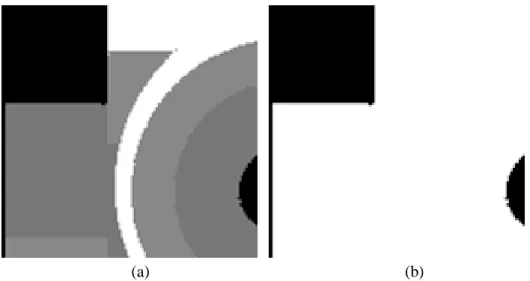
with the maximum value of the aforesaid range. Of a similar way, this happens with addition. By the features of , one can take advantage of its cyclic properties. However, in the current shape in that the images are defined, this is not favorable for our purpose, (see Figure 1). For this reason, the image is redefined in the following way. Let G be an image like a matrix in which the elements belong to the ring , i.e., . As was pointed out previously, the main property acquired by the images, defined in this way, it is the cyclical property under addition and product operations. This property is shown in Figure 2, where it is represented what happens to the gray level values when the addition and multiplication are carried out.

(a) (b)

Figure 1. Effect of multiplying gray level image by a number. (a) Original image, (b) original image multiplied by a large value.

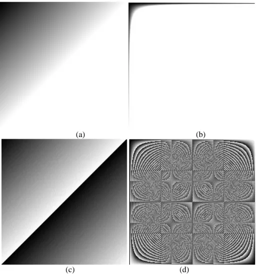
Figure 2 represents an image that characterizes the addition and the multiplication of a gray levels vector in the interval , in this case . One can note that when the operation (addition or multiplication) is carried out with big values, the result in the image greater than 255, it is always forced to be 255. This fact is independently of the values that were used to carry out the operation, and it is a consequence of the necessity of preserving the values of the pixels in the preset interval. Figure 2(a) shows the addition of that vector with the numbers . In Figure 2(b) is represented the product of that vector with the previously mentioned numbers. Note that, one of the main advantages that has the group , it is that when one operates with any two elements of the result is in the interval

64 (a) (b)

(c) (d)

Figure 2. Effect on the gray levels when add and multiply by different values. -axis: gray levels vector in the interval , -axis: gray levels vector in the interval by using the numbers from . (a) Addition and coefficients in , (b) multiplication and coefficients in , (c) addition and coefficients in , (d) multiplication and coefficients in

.

2.4. Comparable and Proportional Images

Definition 1: Comparable images

In the set of images, we will say that two images are comparable if they have the same dimension, i.e.:

Let and be two images and size and respectively, then it is said that are comparable iff and .

Definition 2: Proportional images

Let and be two comparable images, then it is said that and are proportional if exists such that , where , i.e., .

65 Let the symbol represent the relation defined on a set of comparable images such that

are proportional. Then, the relation between and is an equivalence relation.

Two cases in that the images are proportional, and n being not relatively prime integers, takes place when the images are totally homogeneous, or when all the elements that compose the image (pixels) and n are relatively prime integers. In the first case, we are not interested, and the second is not very usual in real images. If the image G is such that all its elements are zeros, then only is proportional to itself. Therefore, if , then is not always ensured the proportionality among images.

Theorem 4: Bijective correspondence of proportional images

If two images are proportional, then their respective sets of gray levels are on bijective correspondence.

The previous theorem specifies that if two images are proportional, then exists a bijective function between them given by the product of the image and a number such that

.

Theorem 5: Entropy of proportional images

If two images are proportional then have the same entropy.

Definition 3: Relative Symmetrical Image

Let two proportional images and be, such that . It is said that an image is the relative symmetrical image of with regard to G by using parameter if

_{, where is the additive inverse of .}

To avoid confusions with the signs of the subtraction operations and subindex notations, starting from this moment to make reference to the symmetrical unit of , it will be used to an scalar element, and – when it is about to a subindex. Note that . The pair of symmetrical images will be denoted by and .

Note that the values and are symmetrical regarding the ring center value. The visual effect in and is that an image is the negative regarding the other one. The result by

product of units has several purposes in depending on the used unit and the image. For example, for we obtain the classical negative image (see Figure 3(a) and 3(d)). For values between 3 and 7 we can highlight the contour for some objects that compose the image (see Figures 3(c) and 3(e)). These values will be used in the next sections for edge detection. However, for large values; for example, greater than 40, the image becomes very noisy (see the third column in the Figure 3). Previous research gave that values greater than 7 make a distortion on contours. For this reason, units values to preserve contours, are on the interval

66

(a) (b) (c)

67 Figure. 3.Symmetrical images. First row: product by small units . Second row: product by

(symmetrical unit of ).

2.5. The gradient operator of the Mean Shift using symmetrical units

In the previous section, the main properties of the units of the rings were exposed with the multiplication operation. In this section, we combine these properties with the Mean Shift in order to produce an image gradient.

Definition 4: Mean Shift of an image

Let be an image, the image that computes the Mean Shift procedure at each point is called the mean shift of . Notation for this application is .

By means of the use of ring units, we use a special notation when Mean Shift vector is applied to an image G that has been multiply by ring units. This element is denoted by , it is given by the following equation:

(3)

Definition 5: Mean Shift Gradient Operator by a Ring Unit

Let G, be an image and a ring unit respectively, the Mean Shift Gradient Operator of G by using , denoted by (Mean Shift Gradient by Ring Units), is defined as:

(5)

In Figure 4, it is shown the image gradient by using applied to a naive binary image made up by a square, where . Note in the first row of this figure, the and

. direction points out from highlighted regions toward dark regions. This is the reason why describes the density from outside toward inside the square, while happens on the contrary with , which describes the density from inside toward out.

68 (a) Original image (b) MSh1 (c) MSh255 (d) MGRU

69 (g) (h)

Figure 4. First row: Images in natural size. Second and third row: increased images (zoom).

Note that, in Figures 4(h), 4(f) and 4(g), MSh values are 0 for those pixels that belong to homogeneous neighborhood. This means that, in the neighborhood of these pixels every neighbor has the same gray level of the central pixel. On the other hand, the zoom image applying MGRU is shown in Figure 4(h). The difference among pixel values that belong to a border and those that not, it is so remarkable that the borders are highlighted. The resulting image highlights the edges of the square.

3.A

In this section, we present our algorithm of the Mean Shift Gradient Operator using Ring Unit ( ). Our algorithm is constituted by three main steps:

1) Filtering

2) The use of Ring Units 3) Thresholding.

70 Result: (Image of edges).

1 Initialize B such that ; 2 Calculate

(according to expression (3));

3 Calculate (according to expression (5));

4 ;

5 Convert to the interval ; 6 Threshold ;

7 Return .

4.

E

R

In this section, we show the experimental results by applying our algorithm. We consider for the experiments two kind of images, the obtained manual segmentation (groundtruth) of the Berkeley database and real images (cerebral hemorrhage images). Attending for each type of image features, we carried out the selection of parameters. For this reason, the parameters were chosen according to a previous analysis of the studied images. Automation of these parameters will be of study in future works.

71

(a) (b)

(c)

(d)

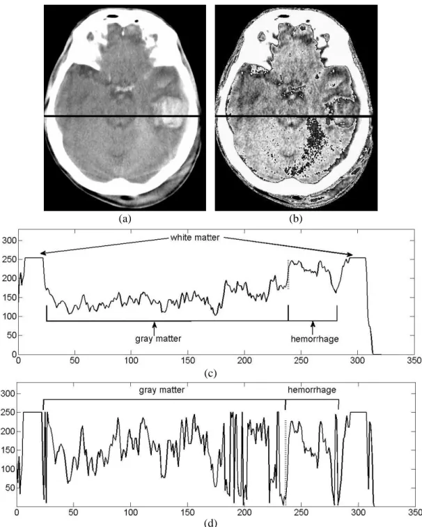
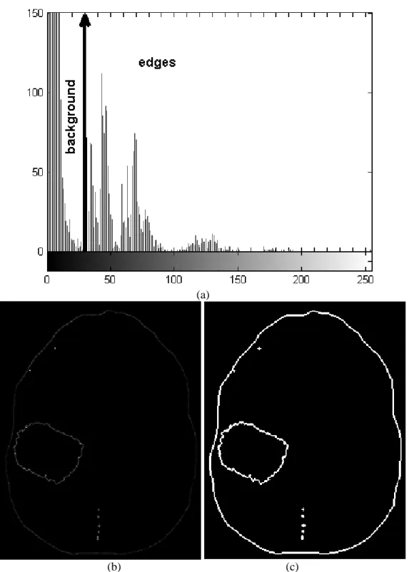
Figure 5. Image profile. (a) Cerebral hemorrhage image. (b) Intensity Profile.

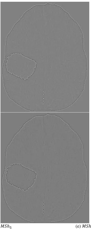
73 (d) (e)

Figure 6. Effect of multiplying by symmetrical units (no filtering step).

74 (a)

(b) (c)

Figure 7. Mean Shift Gradient thresholding of a brain tumor image, without filtering step. 6(a) Histogram. 6(b) After thresholding. 6(c) Before thresholding

75 gaps. The range of threshold for the Canny Edge Detector was [0:0063; 0:0156], out of this interval the image becomes in oversegmentation or undersegmentation. The related results to real images are presented in Figure 9. Note the good obtained results, where so much edges as hemorrhage have been well delimited.

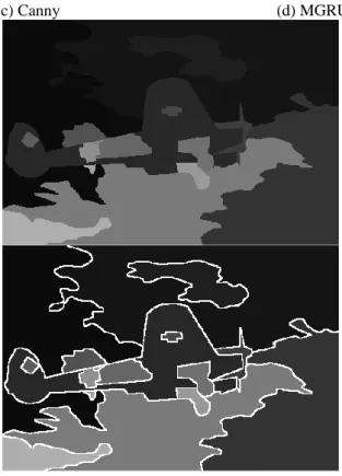
76 (e) Original image (f) Edge superpose

(g) Canny (h) MGRU

78 the Canny edge detection for groundtruth images. Symmetrical ring units were utilized to highlight contour, and the Mean Shift gradient was used for the localization of edges. Several theorem concerning to the ring unit theory applied on images were exposed and proved. Through the obtained results was possible to see that, by using our method, continuous edges were obtained. In future works, the experimental results related to standard and real images will be shown. Also, we will study how to find automatically, the values of the threshold and the unit.

R

[1] Chen, S. & Wang, M., (2005) “Seeking multi-thresholds directly from support vectors for image segmentation”, Neurocomputing, Vol. 67, No. 4, pp335–344.

[2] Cheng~Y., (1995) “Mean Shift, Mode Seeking, and Clustering”, IEEE Trans, Pattern Analysis and Machine Intelligence Neurocomputing, Vol. 17, No. 8, pp790–799..

[3] Comaniciu, D. I., (2000) “Nonparametric Robust Method for Computer Vision”, Ph.D. Thesis, New Brunswick, Rutgers, The State University of New Jersey.

[4] Comaniciu, D. & Meer, P., (2002) “Mean Shift: A Robust Approach toward Feature Space Analysis”, IEEE Transaction on Pattern Analysis and Machine Intelligence, Vol. 24, No. 5. [5] Domínguez, D. & Rodríguez, R.: Use of the L (infinity) norm for image segmentation through

Mean Shift filtering, International Journal of Imaging, Vol. 2, No. S09, pp81–93, 2009.

[6] Fukunaga, K. & Hosteler, D. (1975) “The Estimation of the Gradient of a Density Function”, IEEE Trans., Information Theory, No. 21, pp32–40.

[7] Garces, Y., Torres, E., Pereira, O., Perez, C. & Rodriguez, R., (2013) “Stopping Criterion for the Mean Shift Iterative Algorithm”, Progress in Pattern Recognition, Image Analysis, Computer Vision, and Applications, Springer, Lecture Notes in Computer Science, No. 8258, pp383–390. [8] Garcés, Yasel; Torres, Esley; Pereira, Osvaldo & Rodríguez, (2014) “Roberto Application of the

Ring Theory in the Segmentation of Digital Images”, International Journal of Soft Computing, Mathematics and Control, Vol. 3, No. 4.

[9] Guo, R. & Pandit, S.M., (1998) Automatic threshold selection based on histogram modes and discriminant criterion, Machine Vision and Applications, No. 10, pp331–338.

[10] Grenier, T., Revol-Muller, C., Davignon, F., & Gimenez, G., (2006) “Hybrid Approach for Multiparametric Mean Shift Filtering”, Image Processing 2006, IEEE, International Conference, Atlanta, GA, Vol. 8, No. 11, pp1541–1544.

[11]J ohnson~R.E, (1966) “University Algebra”, Prentice-Hall, Engledwood Cliffs.

[12] Kuo H. W. and Sun Y.N., (2010) “Watershed segmentation with Automatic Altitude Selection and Region Merging Based on the Markov Random Field Model”, International Journal of Pattern Recognition and Artificial Intelligence, Vol. 24, No. 1 , pp153–171.

[13] Loncarics, S., (1998) “A survey of shape analysis techniques”, Pattern Recognition, Vol. 31, No. 8, pp983-1001, 1998.

[14] Osuan-Encison, V., Cuevas, E. & Sossa, H., (2013) “A comparison of nature inspired algorithms for multi-threshold image segmentation”, Expert Systems with Applications, No. 40, pp1213-1219.

[15] Otsu, N., A threshold selection method from gray-level histograms, IEEE Transactions on Systems, Man and Cybernetics, Vol. 9, No. 1, pp62–66.

79 [17] Reza, A.R. & Brewer, V.E., (1989) “Edge Detection Using a Cyclic Ring of Integers Modulo 7”,

IEEE, pp. 145–147.

[18] Rietman, E.A., Karp, R.L. & Tuszynski~J.A., (2011) “Review and application of group theory to molecular systems biology”, Theoretical Biology and Medical Modelling, Vol. 8, No. 21.

[19] Rodriguez R. & Suarez, A. G., (2006) “An Image Segmentation Algorithm Using Iteratively the Mean Shift”, Image Analysis and Applications, Book Progress in Pattern Recognition, Book Series Lecture Notes in Computer Science Publisher Springer Berlin/Heidelberg, Vol. 4225/2006 pp326-335.

[20] Rodriguez R., (2008) “Binarization of medical images based on the recursive application of mean shift filtering: Another algorithm”, Journal of Advanced and Applications in Bioinformatics and Chemistry, , Dove Medical Press Ltd, Vol. I, No. 1:12.

[21] Rodriguez, R., Suarez A. G. & Sossa J. H., (2011) “A Segmentation Algorithm based on an Iterative Computation of the Mean Shift Filtering”, Journal Intelligent and Robotic System, Vol. 63, No.3-4, pp447-463.

[22] Rodriguez, R., Torres E. & Sossa J. H., (2012) “Image Segmentation via an Iterative Algorithm of the Mean Shift Filtering for Different Values of the Stopping Threshold”, International Journal of Imaging and Robotics, Vol. 7, No. 6, pp1–19.

[23] Rodriguez, R., Torres E. & Sossa J. H., (2011) “Image Segmentation based on an Iterative Computation of the Mean Shift Filtering for different values of window sizes”, International Journal of Imaging and Robotics, Vol. 6, No. A11, pp1–19.

[24] Shannon C., A, (1948) “Mathematical Theory of Communication”, Bell System Technology Journal, No. 27, pp370–423.

[25] Shen, D., Horace, H.S., (1997) “A Hopfield neural for adaptive image segmentation: An actice surface paradigm”, Pattern Recognition Letters, No. 18, pp37–48.

[26] Shen, C.& Brooks, M. J., (2007) “Fast Global Kernel Density Mode Seeking: Applications to Localization and Tracking”, IEEE Transactions on Image Processing, Vol. 16, No.5, pp1457-1469.

[27] Suyash, P. A. & Ross T.W., (2006) “Higher-Order Image Statistics for Unsupervised, Information-Theoretic, Adaptive, Image Filtering”, IEEE Transactions on Pattern Analysis and Machine Intelligence, Vol. 28, No. 3, pp364–376.

[28] Venkat, T., Govardhan, A. & Badashah S. J., (2011) “Statistical Analysis for Performance Evaluation of Image Segmentation Quality Using Edge Detection Algorithms”, International Journal of Advanced Networking and Applications, No 03, pp1184–1193.

[29] Wei, C. & Kangling, F., (2008) “Multilevel thresholding algorithm based on particle swarm optimization for image segmentation”, 27th Chinese control conference, Vol.67, No. 4, pp348– 351.

[30] Zhang, D. & Lu G., (2003) “Review of shape representation and description techniques”, Pattern Recognition Society, Published by Elsevier, No. 37, pp1– 19.

[31] Zhiwei, Y., Zhengbing, H., Huamin,. & Hongwei CH., (2011) “Automatic threshold selection based on artificial bee colony algorithm”, 3rd International Workshop on Intelligent Systems and

80 Proof:

Let , be , then we obtain that .

Let be, then , and this means that is a generator of .

Theorem 2: Injectivity of generators of

Let be , .

Proof: Proof by Absurd

Let be, then . Therefore , then is generator of , so the order of is n. It follow that , and this is a contradiction because by hypothesis .

Theorem 3: Equivalence relation of proportional images

Let the symbol represent the relation defined on a set of comparable images such that are proportional. Then, the relation between and is an equivalence relation.

Proof:

Let and be three images defined in a set of comparable images, then:

1) Symmetry

therefore is related to itself, because .

2) Reflexivity

If then , : ,therefore

.

3) Transitivity

If , so , therefore

, where .

But, it is necessary to prove that and n are relatively prime integers, i.e.,

.

If such as

, , then

⁄ and ⁄ , so

81

( ) , therefore

( ).

Consequently, if ( ) and , therefore and n

are relatively prime integers.

Theorem 4: Bijective correspondence of proportional images

If two images are proportional, then their respective sets of gray levels are on bijective correspondence.

Proof:

Let be two proportional images defined in a set of comparable images, then

.

Let { } be the set of gray levels present in the image , i.e.,

, where is the number of gray levels on .

Let { } be the set of gray levels present in the image , i.e.,

, where is the number of gray levels on .

On the other hand, { }1 g, so it satisfies that .

Thefore, by theorems 1 and 2, the sets and are on bijective correspondence.

Theorem 5: Entropy of proportional images

If two images are proportional then have the same entropy.

Proof:

Let and be two proportional images defined in a set of comparable images then,

: .

Let be their respective entropies of , then: ∑ and

∑ .

Let { } be the set of gray levels present in the image . Let

{ } be the set of gray levels present in the image .

.

Equally, it there is a bijective correspondence between the images, and in addition, it there is a one-one correspondence among their sets of gray levels, then the values of the probabilities of occurrence of gray levels do not change. Only change the gray level of these pixels, so: