Hungarian Association of Agricultural Informatics
European Federation for Information Technology in Agriculture, Food and the Environment
Journal of Agricultural Informatics. 2015 Vol. 6, No. 3 journal.magisz.org
Testing of Direct Computer Mapping for dynamic simulation of a simplified
Recirculating Aquaculture System
Mónika Varga1, Sándor Balogh2, Balázs Kucska3, Yaoguang Wei4, Daoliang Li5, Béla Csukás6
I N F O
Received: 23 Aug 2015 Accepted: 23 Sept 2015 Available on-line: 12 Oct 2015 Responsible Editor: M. Herdon
Keywords:
dynamic simulation model, Recirculating Aquaculture System (RAS),
A B S T R A C T
First implementation and testing of Direct Computer Mapping (DCM) based methodology for modeling and dynamic simulation of Recirculating Aquaculture Systems (RAS) were made and evaluated. The test model of the underlying hybrid, multiscale processes were generated for a simplified example system, utilizing data and empirical equations for the production of African catfish (Clarias gariepinus) from the available literature. The Waste Water Treatment model was temporarily implemented by efficiency factor. The authors studied how the graphically generated, locally programmable building elements can be applied for dynamic simulation of the given complex system. According to these previous test results, DCM methodology can give a flexible and robust solution to describe the backbone structure of a core model that can be adapted to the changing formulation and data in the local models, individually. In addition, DCM methodology seems to be able to generate the various RAS schemes from the model of a single fish tank. Based on the experiences, as well as, with the knowledge of a more comprehensive data and relationships, in the ongoing work we shall implement and analyze complex RAS models.
1. Introduction
1.1. Challenge of modeling and dynamic simulation of Recirculating Aquaculture Systems Aquaculture has an increasing role worldwide, providing secure and environmentally benign food for the rapidly growing population (Tacon, 2001). Increasing demand for fish and seafood products exploits the natural resources, so people need more environmentally benign artificial production.
Considering this, the development of sustainable and profitable aquaculture systems needs the application of sophisticated design, planning and control supporting tools. The main challenge in this field is to increase the capacity and to ensure the sustainability in the environment, at the same time. In addition, the development is highly affected by the long term climate change, as well as by the more
1 Mónika Varga
Kaposvár University, Research Group on Process Network Engineering [email protected]
2 Sándor Balogh
Kaposvár University, Research Group on Process Network Engineering [email protected]
3 Balázs Kucska
Kaposvár University, Department of Aquaculture [email protected]
4 Yaoguang Wei
China Agricultural University [email protected]
5 Daoliang Li
China Agricultural University [email protected]
6 Béla Csukás
frequent extreme weather situations. This can be managed only by the utilization of model based design, planning and control methods.
Computational modeling and simulation can highly contribute to the effectiveness of aquaculture systems. Especially, the complex recirculating aquaculture systems (RAS) require simulation model based design and operation, which has initiated an active research field in the past years (e.g. Halachmi et al, 2005; Wik et al, 2009).
Looking at details, in the intensive tanks of the recycling systems the various nutrients, supplied with feed, are converted into valuable product. Considering the sound material balance of the system, many papers focus on the nutrient conversion and on material discharge (Schneider et al, 2004; Verdegem, 2012). Sensor network based monitoring and data collection is a promising field to enhance the productivity and the sustainability of the RAS by minimizing the fresh water supply. Supply chain planning and management of aquaculture products is also a challenging question in the field (Parreño-Marchante et al, 2014; El-Sayed et al, 2015). Several research papers deal with the two-way interaction of aquaculture with environment, in general (McCausland et al, 2006; Grigorakis and Rigos, 2011; Edwards, 2015), or focusing on actual fields (FAO, 2005-2015; Jegatheesan et al, 2011). Up-to-date research works call the attention also to the importance of knowledge transfer and exchange of experience between field experts and policy makers. The importance of well established and conscious regulations (Krause et al, 2015; Alexander et al, 2015) is emphasized, too.
Advanced fish farming can be realized in mainland freshwater and in seaside seawater facilities that are artificially controlled, isolated systems. These isolated systems need maximal recycling of purified water and minimal decontaminated emissions. Also, these isolated systems need disinfected water supply from the environment. Accordingly, these process systems integrate animal breeding with complex bioengineering and other process units in a feedback loop. In addition, the fish production is solved in a stepwise, multistage process, which is also coupled with the characteristics of the life processes (e.g. with the differentiation in growth).
From process engineering point of view, these intensive fish farming technologies are complex hybrid (discrete / continuous), multi-scale process systems with multi-level dynamic behavior, embedding field specific part-processes of multiple disciplines from applied life sciences and engineering. Accordingly, the process design and control need to be supported by respective multidisciplinary computational models.
Process design and control covers the tank structure and the water treatment system, including the removal of solid wastes (e.g. fecal components, feed waste), the conversion of ammonia through nitrite to nitrate (or nitrogen), as well as the supply of dissolved oxygen and the removal of CO2.
1.2. Motivation and objective
The appropriate solutions need sophisticated models, but these models can work only with the knowledge of the detailed, fish specific data. There are and will be more and more data from the sensor networks, and these Big Data, in addition to the data mining of statistical character, ought to be utilized also by the detailed dynamic models. However, the synergic utilization of data based and model based approaches needs robust and flexible models that tolerate the continuous identification with a genetic algorithm, later on.
Considering this, in a small, bilateral Chinese-Hungarian project we decided to start towards applying a non-conventional Hungarian modeling methodology for combining it with the sensor network and data acquisition development of the Chinese partner.
2. Structure and functionalities of RAS
2.1. Structure of RAS
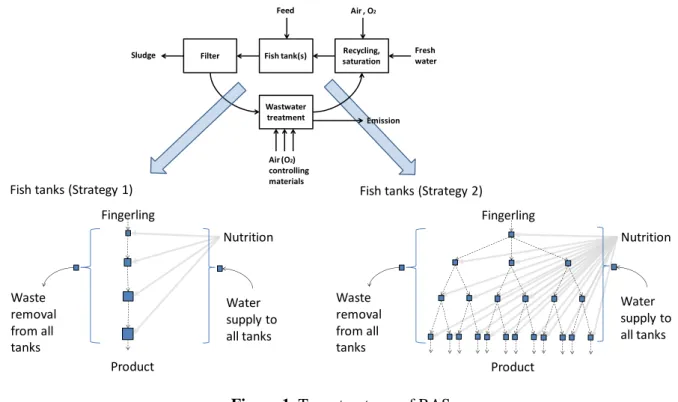
Recirculating Aquaculture Systems can be characterized by the reuse of the effluent water after wastewater filtering and treatment processes, with minimal fresh water supply. A schematic overview of different RASs is illustrated in Fig. 1.
From organizational and modeling point of views, the most difficult part is the fish tank. Considering the tank size and the maximal stocking density, various strategies can be applied during the production cycle. In the lower part of Fig. 1 we introduce two possible arrangements of the fish tanks for the production period. In Scheme 1 there are consecutive, stepwise larger tanks for the increasing fish mass. In Scheme 2, the same sized fish tanks are multiplied along the production period.
Figure 1. Two structures of RAS
2.2. Empirical relationships and data for testing of an example fish tank model
As a comprehensive data set for testing of the model, we utilized the available empirical data and equations for African catfish (Clarias gariepinus) from the course material of Wageningen University (WU, 2014). The example system starts with the stocking of fingerlings with an average of 10 g/piece and ends with an average of 900 g/piece product fish after a 150 days period, with 30 day long harvesting/stocking periods.
Empirical equation for the calculation of the body weight of the given species, determined from long-term experiences, is the following:
(1) 𝐵𝑊 = 0.031 ∗ 𝑋2+ 1.2852 ∗ 𝑋 + 9.4286,
where BW is the body weight of the given fish species in grams X is the age of fish in days
Derived from the long-term production experiences, simple empirical equations can be described for the calculation of other characteristics in the function of the body weight. Accordingly, the following equations were utilized in the model:
Fingerling
Product Waste
removal from all tanks
Water supply to all tanks
Nutrition Nutrition
Waste removal from all tanks
Water supply to all tanks
Fish tanks (Strategy 1) Fish tanks (Strategy 2)
Fingerling
Product Fish tank(s)
Filter saturationRecycling,
Wastwater
treatment Emission
Sludge Fresh
water
Air (O2)
controlling materials
Air , O2
(2) 𝑀𝑜𝑟𝑡𝑎𝑙𝑖𝑡𝑦, % = 57.86 ∗ 𝐵𝑊−0.612, (3) 𝐶𝑜𝑛𝑠𝑢𝑚𝑒𝑑 𝑓𝑒𝑒𝑑 𝑖𝑛 % 𝑜𝑓 𝐵𝑊 = 17.405 ∗ 𝐵𝑊−0.4,
(4) 𝐹𝑒𝑒𝑑 𝑐𝑜𝑛𝑣𝑒𝑟𝑠𝑖𝑜𝑛 𝑟𝑎𝑡𝑒, 𝑔/𝑔 = 0.441 ∗ 𝐵𝑊0.117, (5) 𝐷𝑟𝑦 𝑚𝑎𝑡𝑡𝑒𝑟 𝑖𝑛 % 𝑜𝑓 𝐵𝑊 = 17.267 ∗ 𝐵𝑊0.0778, (6) 𝑃𝑟𝑜𝑡𝑒𝑖𝑛 𝑐𝑜𝑛𝑡𝑒𝑛𝑡 𝑜𝑓 𝑓𝑖𝑠ℎ 𝑖𝑛 % 𝑜𝑓 𝐵𝑊 = 14.372 ∗ 𝐵𝑊0.0234,
where BW is the body weight of the given fish species in grams.
Calculation of metabolic waste emission requires the approximate nutrient composition. According to the example diet composition, we calculated with the following concentrations of components:
490 g/kg protein,
120 g/kg fat,
233 g/kg carbohydrate,
77 g/kg ash,
altogether 920 g/kg dry matter.
Organic matter content can be quantified as Chemical Oxygen Demand (COD). In the referred example system authors give empirical numbers for converting food components into COD as follows:
protein: 1.25 g COD/g nutrient,
fat: 2.9 g COD/g nutrient,
carbohydrate: 1.07 g COD/g nutrient.
3. Direct Computer Mapping of a simplified test model
As we introduced it in our former papers (e.g. Varga et al, 2015), Direct Computer Mapping (DCM) is a continuously evolving, general methodology for modeling and simulation of various kinds of agricultural and environmental process systems. Having recognized the need for a general purpose process modeling methodology, in this approach (Csukas et al, 2011) we map the elements and their connections onto an executable computational model without using any specific single mathematical apparatus. In the recent development of DCM we synthesized the experiences coming from the analysis of a broad range of processes from cellular biosystems (Csukas et al, 2013.a.) through technological process units (Csukas et al, 2013.b.) to sector spanning agri-food process networks (Varga et al, 2010; Varga et al, 2012). Based on these examples, a general set of building and connecting elements was recognized, which have the capability to implement a broad range of process models from quite different fields. Accordingly, the complex structures and functionalities of the various continuous and discrete, as well as quantitative and qualitative process models can be mapped onto the same, unified state, transition and connection elements, while the elements are associated with locally executable programs. It is to be noted, that the applied modeling methodology makes possible the flexible replacement of the whole model, including the equations and the data, within the implemented structure.
Model building procedure can be generalized as follows:
1. Editing of the model structure according to the flow sheet of the process system to be investigated;
2. Transformation of flow sheet elements into simple network; 3. Formulation of state and transition prototypes of the DCM model; 4. Transformation of the simple network into the DCM net model; 5. Parameter setting;
Recently, we have been applied the method for the model based investigation of meteorological effects on a sensitive watershed. The description of the up-to date modeling framework and applied software components are described in detail in our previous publications (Varga et al, 2015).
3.1. Implementation of a simplified RAS model into a DCM
In this work, possible implementation of a simplified RAS model in the DCM simulator has been tested.
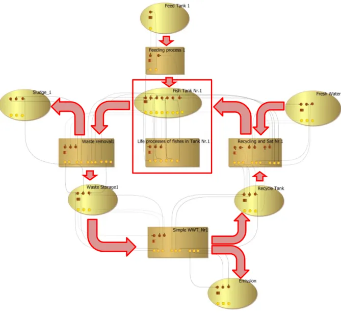
In line with the principles of DCM, model building starts from the determination of state and transition prototype elements for the investigated process system. Accordingly, we defined the prototypes, and utilized the general set of DCM building blocks to describe a simplified RAS model according to Fig. 2.
Figure 2. DCM based implementation of the simplified RAS model
The state describing prototype elements are the followings:
feed tank,
fish tank, containing slots for feed, air (oxygen) liquid, solid and various fish components,
sludge,
general liquid storage tank (intermediate),
general liquid storage tank (terminal).
life processes of fishes,
feeding process,
waste removal,
wastewater treatment,
recycling and saturation.
Fig. 2 shows the test model of the RAS cycle, built from the above mentioned state and transition prototype elements. In line with the recent developments of DCM method (Varga et al, 2015), we used the yEd graph based expert interface for the structural and functional editing of the model. In DCM model the material flows are represented by increasing (solid) and decreasing (dashed) connections between the respective slots of the given elements, while dotted lines correspond to the forwarding of the data, used in the calculation of the local programs. The material flows are indicated also by better visible arrows in the Figure.
3.2. Description of "fishtank" and "lifeprocess" prototypes
In the following we discuss the state element “fish tank” and the transition element “life processes” in more detail.
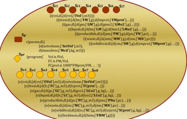
The fish tanks (represented by a couple of the above state and transition elements) are the main parts of the RAS, where fishes are growing during the production period. All of the life-related processes are linked to this unit. Besides the respiration, excretion and other life-related processes, fishes transform the feed partly into body mass, according to the feed conversion rate. Other parts are going to waste. To describe these functionalities in the model, in line with DCM method, the prototype element contain input slots (signed with Si1 – Si7 in Fig. 3) for volume, m3; feed, g; gas, g; liquid, g; product fish, g; waste, g; and solid (fecal) parts, g phases. Parameter slot of fish tank element (signed with Sp in Fig. 3) is responsible for the control of the desired tank volume (setvolume, m3), as well as for the prescribed maximal stocking density (maxdens, kg/m3). Output slots (signed with So1 – So8 in Fig. 3) are similar to input slots. They are responsible for forwarding the concentrations, calculated by the local program that utilizes the data coming from input and parameter slots. Additionally, the model of the fish tank contains an extra slot for the calculated amount of feed requirement (So8 in Fig. 3).
In building of model structure, we utilize the prototypes to generate the actual elements from them. Actual elements contain the same input, parameter and output slots, as well as a reference for the calculating program given in the prototype name. In case of actual elements, we replace the input and parameter variables (highlighted with bold in Fig. 3) for the actual values.
Figure 3. Zooming into the model of fish tank
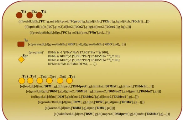
The life process describing transition prototype element contains input slots for feed, g/m3; liquid, g/m3; and productfish, g/m3 (signed with Ti1 – Ti3 in Fig. 4). Differentiation in growth of fishes during the production period is a general operational problem of RAS. To consider this feature in the model correctly, we added a parameter slot for describing the different growing abilities, divided the population into three categories (normal, undersized and oversized) (Spr in Fig. 4). As an example, for the distribution we assumed that 68% of fishes belong to the normal category. Output slots provide places for calculated values of feed, g; gas, g; liquid, g; product fish, g; waste, g; and solid (fecal) parts, g (signed with To1 – To6 in Fig. 4).
Calculation of the values for output slots is determined by the actual values of input and parameter slots, as well as by the empirical equations (right now from the literature, see in Chapter 2.2). It is to be noted, that for testing of the model we used the previously shown heuristic equations, but in a more sophisticated model these expressions can be replaced easily for other, more comprehensive and well-tested ones.
c(param,dl,[
[d(setvolume,['SetVol'],m3), d(maxcdens,['Mcd'],kg_m3)]) {program(' Vol is IVol,
FC is FM/Vol,
FCprot is 1000*FMprot/FM, … .')} Spr
Sp
A state prototype: Fish tank {e(p,y,fish_tank,[],fish_tank,[],[],[])}
Si4 Si5 Si6 Si7
{o(feed,dl,[d(fc,['FC'],g_m3),d(fcprot,['FCprot'],…])} Si1 Si2 Si3
{i(feed,dl,[d(fm,['FM'],g),d(fmprot,['FMprot'],…])} {i(gas,dl,[d(gm,['GM'],g),d(gmo2,['GMo2'],g),…)])}
{i(liquid,dl,[d(lm,['LM'],g),d(lmo2,['LMo2'],g), …])}
{i(waste,dl,[d(mm,['MM'],g),d(mn,['MN'],pc)])} {i(productfish,dl,[d(pm,['PM'],g),d(pn,['PN'],pc), …])}
{i(solidfecal,dl,[d(sm,['SM'],g),d(smprot,['SMprot'],g), …])}
So1 So2 So3 So4 So5 So6 So7
{o(gas,dl,[d(gc,['GC'],g_m3),d(gco2,['GCo2'],g_kg), …])} {o(liquid,dl,[d(lc,['LC'],g_m3),d(lco2,['LCo2'],g_kg), …])}
{o(waste,dl,[d(mc,['MC'],g_m3),d(mn,['MN'],pc) …])} {o(productfish,dl,[d(pc,['PC'],g_m3),d(pnu,['PNu'],pc), …])}
{o(solidfecal,dl,[d(sc,['SC'],g_m3),d(scprot,['SCprot'],g_kg), …])} {o(vol,dl,[d(vol,['OVol'],m3),d(setvolume,['SetVol'],m3)])}
{i(vol,dl,[d(vol,['IVol'],m3)])}
So8
Figure 4. Zooming into the model of life processes
4. Test results of the simulation model
In this first simulation trial we simulated a single example fish tank in the RAS cycle. In line with the investigated case, we show the results for the second 30 days long period, followed after the previous simulation of the first 30 days. The technological parameters were the followings:
volume of fish tank: 3 m3,
number of fishes: 6000 pieces,
average starting weight if fishes: 10 g,
stocking density of fishes in second stage: 140 - 360 kg/m3,
controlled nutrition level: 30 kg/m3,
water exchange: 3 m3/day,
efficiency of dentrification: 0.95,
fresh water supply: 20%.
Having determined and generated the DCM model structure for the example RAS, we adjusted the parameters of the model according to the example system, described in Section 2.2.
In the simulation results, we can monitor the following characteristics:
growth of fish and stocking density in fish tank,
mortality of fishes during the simulation period,
liquid and solid components in fish tank,
amount of sludge and its solid and liquid components,
wastewater's solid and liquid components (before treatment),
emission of solid and liquid components,
recycle's solid (COD and ash), and liquid components,
fresh water supply.
In the following diagrams we illustrate some examples for the simulated results. {c(param,dl,[d(growthdiffu,['GDU'],nd),d(growthdiffo,['GDO'],nd),…])}
Spr
Tp
A transition prototype: Life processes {e(a,y,lifeprocesses,[],lifeprocesses,[],[],[])}
{o(gas,dl,[d(gm,['DGM'],g),d(gmo2,['DGMo2'],g),d(gmco2,['DGMco2'],g),d(gmn2,['DGMn2'],g)])}
Ti1 Ti2 Ti2
{i(liquid,dl,[d(lc,['LC'],g_m3),d(lco2,['LCo2'],g_kg),d(lcco2,['LCco2'],g_kg),..])} {i(productfish,dl,[d(pc,['PC'],g_m3),d(pnu,['PNu'],pc),…])}
To1 To2 To3 To4 To5 To6
{o(liquid,dl,[d(lm,['DLM'],g),d(lmo2,['DLMo2'],g),d(lmco2,['DLMco2'],g),…])} {o(productfish,dl,[d(pm,['DPM'],g),d(pn,['DPN'],pc),d(pmu,['DPMu'],g),…)])}
{o(solidfecal,dl,[d(sm,['DSM'],g),d(smprot,['DSMprot'],g),d(smfat,['DSMfat'],g),…])} {o(waste,dl,[d(mm,['DMM'],g),d(mn,['DMN'],pc)])}
{o(feed,dl,[d(fm,['DFM'],g),d(fmprot,['DFMprot'],g),d(fmfat,['DFMfat'],g),d(fmch,['DFMch'],…])} {i(feed,dl,[d(fc,['FC'],g_m3),d(fcprot,['FCprot'],g_kg),d(fcfat,['FCfat'],g_kg),d(fcch,['FCch']),…])}
In the following example we zoomed into a 30 days long simulation period (from the 30th to 60th days) of the 150 days long production period. To study also the above mentioned differentiation in growth of fishes, we distinguished three groups of them, i.e. the normal, the undersized and the oversized group. We assumed, that about 1616% of the fishes belongs to the under and oversized groups, with -+ 1 g difference in the average starting weight, respectively.
Fig. 5 shows the changes in the fish population within the 30 days long simulation period. The decrease depends on mortality, as well as in line with equation (2), rate of mortality is determined by the body weight. In the three groups the number of fishes (starting originally from 1000, 4000 and 1000 pieces) decreases in line with the cumulated mortality (green line belongs to the right side scale).
Figure 5. Number of fishes
At the beginning of the investigated simulation stage (from the 30th day of the production period), fingerlings’ individual body weight is around 40 g. Fig. 6 shows the increase in body weight, where the average sizes of product fish in the undersized, normal and oversized groups increase to 90, 110 and 140 g until the end of the given period (60th day of the production), respectively.
Figure 6. Average individual weight in the three groups
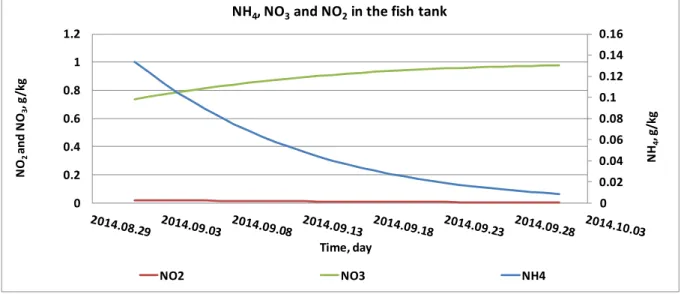
Life processes (especially energy production, associated with the catabolic processes) consume O2 and produce CO2 and NH4. NH4 and its decomposition products in the wastewater treatment (NO2, NO3) can be toxic for fishes. Consequently, they have to be removed by wastewater treatment, as well as have
3885 3890 3895 3900 3905 3910 3915 3920 3925 3930 968 970 972 974 976 978 980 982 984 N u m b e r o f fi sh e s in u n d e r-an d o ve rs iz ed gr o u p , p ie ce Time, day
Number of fishes in the three groups
Number of fishes in the undersized group, pc Number of fishes in the oversized group, pc
Number of fishes in the normal group, pc
N u m b e r o f fi sh e s in t h e n o rm al gr o u p , p ie ce 0 20 40 60 80 100 120 140 160 A ve ra ge in d ivi d u al w e igh t, g Time, day
Average individual weight in the three groups
to be decreased by fresh water supply. Frequent monitoring of these components has a keynote role in aquatic production systems. Fig. 7 shows the simulated amount of these key monitoring parameters (ammonium, nitrite and nitrate).
Figure 7. Concentration of some dissolved nitrogen containing components in the fish tank
The sludge (with a given moisture content) is removed from the system by filtering. Other parts of the waste go toward the wastewater treatment. Emissions leaves the system after the treatment and one part of treated wastewater goes to the recycle tank for re-utilization. This amount, together with the necessary freshwater, returns to the fish tank after saturation with oxygen from air of increased pressure.
5. Conclusions and ongoing future work
Considering the role of aquaculture in the future’s quantitative and qualitative food security, the use of advanced decision support systems, as well as design and control algorithms are inevitable in development of Recirculating Aquaculture Systems. Dynamic simulation can highly contribute to the planning and effective operation of RAS. Considering the complexity of the underlying hybrid, multiscale processes, the appropriate solution, it is worth to try the applicability of the new modeling and simulation methodologies.
The appropriate models can work only with the knowledge of the detailed, fish specific data. In contrary, there are more and more available data (e.g. from sensor networks), and these Big Data ought to be utilized also for the identification of the detailed dynamic models. However the synergistic utilization of data based and model based approaches needs robust and flexible models that tolerate the continuous identification (e.g. with a genetic algorithm), later on. Considering this, in a bilateral Chinese-Hungarian project we decided to start toward combining a non-conventional Hungarian modeling methodology with the sensor network based data acquisition of the Chinese partner.
In this paper the first step toward the implementation and testing of a Direct Computer Mapping based methodology for modeling and dynamic simulation of Recirculating Aquaculture Systems is illustrated. The test model of the underlying processes was generated for a simplified example system, utilizing data and empirical equations for the production of African catfish (Clarias gariepinus) from the literature. The Waste Water Treatment model was temporarily implemented by efficiency factors.
We concluded that the graphically generated, locally programmable building elements of DCM can be applied for dynamic simulation of the given complex systems. According to the results, DCM methodology gives a flexible and robust solution to describe the backbone structure of a core model that can be adapted to the changing formulation and data of the local models, with no restriction for any
0 0.02 0.04 0.06 0.08 0.1 0.12 0.14 0.16
0 0.2 0.4 0.6 0.8 1 1.2
NO
2
an
d
N
O3
, g
/k
g
Time, day
NH4, NO3and NO2in the fish tank
NO2 NO3 NH4
NH
4
, g/
single mathematical apparatus. In addition, DCM methodology seems to be able to generate various, complex RAS schemes from the model of a single fish tank. The method can consider also the differentiation in weight of fishes.
Based on the experiences and, with the knowledge of a more comprehensive set of data and relationships, in the ongoing work the implementation of complex RAS models is aimed, which can be improved by the accumulating data acquisition based knowledge.
Acknowledgement
The research was funded by TÉT_12_CN-1-2012-0041 and partly by TÁMOP 4.2.1.C-14/1/KONV-2015-0008 projects.
References
Alexander, K.A., Potts, T.P., Freeman, S., Israel, D., Johansen, J., Kletou, D., Meland, M., Pecorino, D., Rebours, C., Shorten, M., Angel, D.L. 2015. The implications of aquaculture policy and regulation for the development of integrated multi-trophic aquaculture in Europe. Aquaculture, 443: 16-23. doi:
10.1016/j.aquaculture.2015.03.005
Csukas, B., Varga, M., Balogh, S. 2011. Direct Computer Mapping of Executable Multiscale Hybrid Process Architectures. In: Proceedings of Summer Simulation Multiconference’2011, Den Haag. Hollandia, 2011.06.26-2011.06.29. pp. 87-95.(ISBN:1-56555-345-4)
Csukas, B, Varga, M, Prokop, A. 2013.a. Direct Computer Mapping Based Modeling of a Multiscale Process Involving p53/miR-34a Signaling. In: Prokop A, Csukás B (eds.) Systems Biology: Integrative Biology and Simulation Tools. Dordrecht: Springer Science+Business Media, pp. 497-548. ISBN:978-94-007-6802-4, doi:
10.1007/978-94-007-6803-1_18
Csukas B, Varga M., Miskolczi N., Balogh S., Angyal A., Bartha L. 2013.b. Simplified Dynamic Simulation Model of Plastic Waste Pyrolysis in Laboratory and Pilot Scale Tubular Reactor. Fuel Processing Technology, 106: 186-200., doi: 10.1016/j.fuproc.2012.07.024
Edwards, P. 2015. Aquaculture environment interactions: Past, present and likely future trends. Aquaculture. In Press, Corrected Proof, Aailable online 11 February 2015.
El-Sayed, A-F.M., Dickson, M.W., El-Naggar, G.O. 2015. Value chain analysis of the aquaculture feed sector in Egypt. Aquaculture, 437: 92-101., doi: 10.1016/j.aquaculture.2014.11.033
FAO 2005-2015. World inventory of fisheries. Impact of aquaculture on environment. Issues Fact Sheets. Text by Uwe Barg. In: FAO Fisheries and Aquaculture Department (online). Rome. Updated 27 May 2005. (Cited 20 April 2015). http://www.fao.org/fishery/topic/14894/en
Grigorakis, K., Rigos, G. 2011. Aquaculture effects on environmental and public welfare – The case of Mediterranean mariculture. Chemosphere, 85(6): 899-919., doi: 10.1016/j.chemosphere.2011.07.015
Halachmi, I., Simon, Y., Guetta, R., Hallerman, E.M. 2005. A novel computer simulation model for design and management of re-circulationg aquaculture systems. Aquacultural Engineering, 32: 443-464., doi:
10.1016/j.aquaeng.2004.09.010
Jegatheesan, V., Shu, L., Visvanathan, C. 2011. Aquaculture Effluent: Impacts and Remedies for Protecting the Environment and Human Health. Reference Module in Earth Systems and Environmental Sciences,
Encyclopedia of Environmental Health. 123-135., doi: 10.1016/b978-0-444-52272-6.00340-8
Krause, G., Brugere, C. Diedrich, A., Ebelingf, M.W., Ferseh, S.C.A., Mikkelseni, E., Pérez Agúndezj, J.A., Steadk, S.M., Stybell, N., Troellm, M. 2015. A revolution without people? Closing the people–policy gap in aquaculture development. Aquaculture, In Press, Corrected Proof, Available online 14 February 2015., doi:
10.1016/j.aquaculture.2015.02.009
McCausland, W.D., Mente, E., Pierce, G.J., Theodossiou, I. 2006. A simulation model of sustainability of coastal communities: Aquaculture, fishing, environment and labour markets. Ecological Modelling, 193(3–4): 271-294., doi: 10.1016/j.ecolmodel.2005.08.028
Schneider, O., Sereti, V., Eding, E.H., Verreth, J.A.J. 2004. Analysis of nutrient flows in integrated intentensive aquaculture systems. Aquaculturel Engineering, 32: 379-401., doi: 10.1016/j.aquaeng.2004.09.001
Tacon A.G.J. 2001. Increasing the contribution of aquaculture for food security and poverty alleviation. Technical Proceedings of the Conference on Aquaculture in the Third Millennium.
(http://www.fao.org/docrep/003/AB412E/ab412e30.htm).
Varga, M., Balogh, S., Csukás, B. 2010. Sector spanning agrifood process transparency with Direct Computer Mapping. Agricultural Informatics. 1(2): 73-83., doi: 10.17700/jai.2010.1.2.22
Varga M, Csukas B, Balogh S. 2012. Transparent Agrifood Interoperability, Based on a Simplified Dynamic Simulation Model. In: Mildorf T, Charvat K (eds.) ICT for Agriculture, Rural Development and Environment: Where we are? Where we will go? Prague: Czech Centre for Science and Society, pp. 155-174. ISBN: 978-80-905151-0-9
Varga, M., Balogh, S., Csukás, B. 2015. Preparation of a dynamic simulation model to support decision making in a shallow lake area. Journal of Agricultural Informatics, 6(1): 11-23., doi: 10.17700/jai.2015.6.1.159
Verdegem, M.C.J. Nutrient discharge from aquaculture operations in function of system design and production environment. Reviews in Aquaculture, 4: 1-14., doi. 10.1111/raq.12011
Wik T.E.I., Lindén, B.T., Wramner, P.I. 2009. Integrated dynamic aquaculture and wastewater treatment modelling for recirculating aquaculture systems. Aquaculture, 287: 361-370., doi:
10.1016/j.aquaculture.2008.10.056