Hardware-Software Co-design for Reconfigurable Field Programmable Gate
Arrays Using Mixed-Integer Programming
Faridah M. Ali
Department of Computer Engineering,
Kuwait University, P.O. Box 5969, Safat 13060, Kuwait E-mail: [email protected]
Helal Al-Hamadi
Department of Information Science,
Kuwait University, P.O. Box 5969, Safat 13060, Kuwait E-mail: [email protected]
Ahmed Ghoniem
Department of Finance and Operations Management,
Isenberg School of Management, University of Massachusetts Amherst, Amherst, MA 01002, U.S.A.
E-mail: [email protected]
Hanif D. Sherali
Grado Department of Industrial and Systems Engineering (0118), Virginia Tech,
Blacksburg, VA 24061, U.S.A. E-mail: [email protected]
Keywords:hardware-software co-design, FPGAs, task partitioning, scheduling, mixed-integer 0-1 programming
Received:September 19, 2011
This paper presents a novel mixed-integer programming formulation for scheduling non-preemptive, aperi-odic, hard real-time tasks with precedence constraints. It provides an integrated partitioning and scheduling co-synthesis approach. The problem formulation maps somenprecedence-related, indivisible jobs hav-ing specified processhav-ing requirements, release times, and due-dates to a system involvhav-ing a shav-ingle Central Processing Unit (CPU) and up tompotential reconfigurable Field Programmable Gate Arrays (FPGAs). We provide a time-indexed mixed-integer 0-1 programming formulation that jointly assigns tasks to either the CPU or to one of the FPGAs, and determines the task sequence for each software or hardware compo-nent that is utilized, with the objective of minimizing a composite cost of task partitioning and scheduling. Computational experience is provided using randomly generated instances to demonstrate the applicability of the proposed methodology.
Povzetek: Predstavljen je algoritem za porazdeljevanje opravil pri snovanju programske in strojne opreme.
1
Introduction and Motivation
The task partitioning and scheduling problem bears prac-tical significance in software/hardware co-design of hard real-time applications that arise in a host of applications such as flight and defense control, telecommunication, or nuclear power plants, to name a few. Specifically, we con-sider the problem of partitioning and schedulingn indivisi-ble (no preemption), aperiodic (which could be considered as the body of a looped system), precedence-related jobs that are characterized by specific processing requirements, release times, and due-dates (which are deadlines that
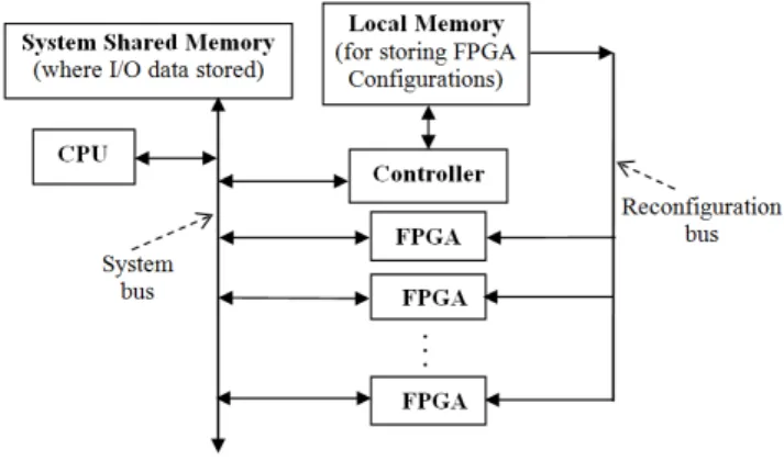
Figure 1: System Architecture
that arise in production and logistical systems where it is often desirable to meet imposed due-dates, it isimperative to comply with the specified due-dates in the problem un-der investigation.
Another reason for the use of such dual systems in prac-tice resides in the benefits accruing from the cooperation between software and hardware components. As a conse-quence, the co-design problem has gained increasing at-tention over the last decade, (see [6], [7], [10], [12], [16], [19], and [20]). This process involves three main oper-ations, namely, resource (software, hardware, and auxil-iary components)allocationto the system, task partition-ingamong software and hardware processing components, andschedulingof the tasks over their assigned processing components (CPU or FPGA). Most works in the literature have addressed this joint problem via two-phase methods [14], where a task partitioning is achieved first, and then tasks are subsequently scheduled over the relevant process-ing components. It is important, however, to note that the task partitioning and scheduling operations are intertwined [9], and need to be dealt with concurrently in order to de-termine optimal operational solutions.
An algorithm that aims at partitioning and scheduling the tasks on two CPUs and several hardware components with the objective of minimizing the total execution time and the hardware cost was presented by Liu and Wong [13]. Arato et al. [2] designed a procedure for schedul-ing tasks on a software component, where tasks that violate their deadlines are partially assigned to an auxiliary hard-ware component. A mixed-integer 0-1 formulation for par-titioning precedence-related tasks on a single-CPU-single-FPGA system, as well as a genetic algorithm to address larger problem instances was presented in [2]. Ali and Das [1] presented a heuristic algorithm that progressively as-signs indivisible tasks to dynamically reconfigurable FP-GAs when certain tasks cannot meet their deadlines on the CPU. In contrast, this challenging scheduling problem is tackled in the present paper using a mixed-integer 0-1 pro-gramming model with the objective of minimizing a com-posite cost of task partitioning and scheduling on a single CPU along with several potentially reconfigurable FPGAs.
Jeong et al. [11] proposed a mixed-integer 0-1 formu-lation and a heuristic for hardware-software partitioning in systems consisting of a single CPU and a single FPGA, with the objective of minimizing the reconfiguration over-head. A mixed-integer programming model was developed by Niemann and Marwedel [14] that employs a two-phase method for hardware/software partitioning, where a tenta-tive schedule is first proposed and is subsequently verified; if the timing constraints are violated, the partitioning step is repeated with timing constraints that are tighter than the es-timated scheduling horizon length. Bender [3] discussed an alternative mixed-integer programming approach for map-ping real-time precedence graphs into a system of Appli-cation Specific Integrated Circuits (ASICs) that are used as hardware components, and pipelined microprocessors that are used as software components. Initially, only a limited number of hardware components are used, and these are in-crementally increased until a feasible solution is obtained.
Recently, hardware/software partitioning for multimedia and wireless mobile applications has gained great impor-tance. Brogioli et al. [4] proposed a set of criteria for partitioning real-time embedded multimedia applications between software programmable Digital Signal Processors (DSPs) and hardware-based FPGA coprocessors. Dasu and Panchanathan [5] investigated the design and development of a dynamically reconfigurable multimedia processor that involves an optimal hardware/software codesign method-ology. Furthermore, a hardware/software partitioning for multimedia application that utilizes process-level pipelin-ing and a heuristic technique based on simulatpipelin-ing annealpipelin-ing was presented by Juan et al. [12].
A design space exploration tool that supports both ex-plicit communication and reconfigurable hardware was ad-dressed by Haubelt et al. [10]. The developed algorithm strictly separates functionality from the architecture, and maps a process graph onto components such that data de-pendencies given by the process graph can be handled in the resulting implementation. The work presented in the present paper bears some similarity to this approach in that we also use explicit communication channels and reconfig-urable hardware in our system architecture.
Observe that the problem at hand is also related to the challenging class of unrelated parallel machine schedul-ing problems (see [15]). It is characterized by the pres-ence of release dates, imperative due-dates, precedpres-ence constraints, inter-task data communication, reconfiguration of hardware resources (FPGAs), and a composite objective function that minimizes the processing and resource uti-lization costs. Also, it is specially structured due to the fact that all processing components are identical, except for the CPU.
scheduling tasks onto hardware/software units, and second, it offers a design space exploration tool to ascertain the minimum number of FPGAs required for a particular ap-plication before a system is actually built.
The remainder of this paper is organized as follows. In Section 2, we formally describe the problem under inves-tigation along with our notation. Thereafter, we introduce in Section 3 a mixed-integer 0-1 programming formulation that simultaneously captures the requirements pertaining to the partitioning and scheduling operations. Section 4 delin-eates our data generation scheme, and reports our compu-tational experience using a set of random test instances to demonstrate the effectiveness of the proposed solution ap-proach. We close the paper in Section 5 with a summary of our findings.
2
Problem Description and Notation
We address the problem of scheduling somen precedence-related jobs having specified processing requirements, re-lease times, and inviolable due-dates in a system involving a singleCentral Processing Unit(CPU) and a maximum of somempotential reconfigurableField Programmable Gate Arrays(FPGAs). Each job can be processed either by the CPU itself, or it can be scheduled for processing on one of the mavailable FPGAs. In either case, no preemption is permitted, and each resource (CPU or FPGA) can process at most one job at any point in time. However, whenever an FPGA begins processing a job, it must be reconfigured to perform the required operation by a single available re-configurationcontroller. This reconfiguration process con-sumes a specified duration that is part of the total process-ing time required for performprocess-ing the job on the associated FPGA. Note that while the controller is reconfiguring any FPGA to begin processing a job, it is occupied and cannot simultaneously reconfigure another FPGA. Again, no pre-emption is permitted in the reconfiguration process. Also, not all themavailable FPGAs need be used; in fact, there is a fixed cost for using an FPGA that competes with the cost related to achieving scheduling efficiency. When an FPGA finishes executing any task, it becomes available for the next task if needed. This is described more in detail in the model formulation given in Section 3.
In our analysis, the FPGAs cannot be preconfigured since it is not known in advance which task will be exe-cuted on the FPGA rather than on the CPU. Moreover, if the system has more than one FPGA, it is not known which FPGA will be used until scheduling is complete. The pro-posed system (Figure 1) is generic and can be used for ex-ecuting any precedence-related jobs. However, for a given real-time set of jobs, once an optimal system configuration and scheduling decisions are determined, then a partial run-time reconfiguration can be performed during implementa-tion where only the configuraimplementa-tion bits of the particular task are transferred to the FPGA in order to reduce the configu-ration time.
Notation:
– j= 1, ..., n: Index for jobs.
– For establishing precedences, we define P =
{(j1, j2) :j1→j2, i.e., the processing of jobj1must
precede that of jobj2}.
– m=maximum potential number of FPGAs available for use.
– Index fortime-slots: Let the time be discretized so that the scheduling time-line for the CPU and each FPGA contains s time-slots, where the end of time-slot s is estimated to be the maximum allowable makespan duration, based on due-dates. We index the time-slots over this maximum makespan duration as: t = 1, ..., s. (Note that the actual duration of the time-slots is arbitrary and rescalable, and typically ranges from 1 to 300 seconds in practice. Also, the time measure-ment (in discretized units) begins at timet= 0at the beginning of slot 1.)
– Index forslots: These correspond to a sequential in-dexing of the foregoing time-slots over the resources, where the slots for the CPU are indexed as k = 1, ..., s, the slots for FPGA 1 are indexed as k =
s + 1, ...,2s, the slots for FPGA 2 are indexed as k = 2s + 1, ...,3s, and so on, up to slots k =
ms+ 1, ...,(m+ 1)s for FPGA m. (Note that the time-slotsare numbered1, ..., s, whereas theslotsare indexed contiguously over the CPU and themFPGAs ask= 1, ...,(m+ 1)s.)
– Index for resources: r = 0,1, ..., m, wherer = 0is the CPU andr= 1, ..., mindex the FPGAs.
– r(k) =resource corresponding to slotk. (Sor(k) = 0
fork= 1, ..., s,r(k) = 1fork=s+ 1, ...,2s, and so on.)
– δjr =processing time of jobjon resource r(in
in-tegral time units that conform with the time-slot dura-tion).
– πjr= reconfiguration time on resource FPGArto
pro-cess jobj(in integral time units that conform with the time-slot duration). We assume thatπjr is included
withinδjr,∀j,∀r≥1.
– αj =release time of job j. That is, if a job j has
no predecessors, then the earliest time-slot to start its processing isαj+ 1.
– dj=due-date of jobj.
– lbj = lower bound on the starting time-slot for job
j. If a job has no predecessor, then lbj = αj + 1;
otherwise we may simply take lbj = max{αj +
1, max
j1:(j1,j)∈P
– kmod+(s) =remainder for the divisionk/s, except that this is taken assif the remainder is zero.
Principal Decision Variables:
The principal decision variables are defined below:
– xjk=
{
1 if job j is assigned to start at slot k
0 otherwise, ∀j, k.
– yr=
{
1 if FPGA r is utilized
0 otherwise, r= 1, ..., m.
Auxiliary Decision Variables:
The following auxiliary variables are defined based on thexjk-variables:
– sj =time-slot at which the processing of jobjstarts.
– fj =time-slot at which the processing of jobjends.
Key Sets:
We define certain key sets based on individual job pro-cessing times (which could, in general, be CPU- and FPGA-dependent), reconfiguration times (which could again be FPGA-dependent), job release/availability times, and job due-dates:
– Sj ≡{slotsk: xjk = 1is a possible decision based
on release, due-date, processing, and reconfiguration times},∀j = 1, ..., n.
Observe that we may expressSjas
Sj ={k:k∈ {1, ...,(m+ 1)s}, lbj≤kmod+(s)≤
dj−δjr(k)+ 1},∀j = 1, ..., n.
– Sjr = {k ∈ Sj :
slotkis associated with resourcer},∀j = 1, ..., n, r= 0, ..., m.
– Jk = {(j, ℓ) : j ∈ {1, ..., n}, ℓ ∈ Sj, andxjℓ = 1
would imply that slotkwould be occupied by the re-configuration/processing of jobj},∀k = 1, ...,(m+ 1)s.
Note thatJkcan be expressed as
Jk = {(j, ℓ) : j ∈ {1, ..., n}, ℓ ∈ Sj, r(ℓ) =
r(k), ℓmod+(s) ≤ kmod+(s) ≤ ℓmod+(s) +
δjr(ℓ)}.
– Rt = {(j, ℓ) : j ∈ {1, ..., n},ℓ ∈ Sj, andxjℓ = 1
would imply that during the time-slott, the controller is busy performing a reconfiguration},∀t= 1, ..., s−
∆, where∆ = min
j,r {δjr−πjr}.
We can formally stateRtas
Rt = {(j, ℓ) : j ∈ {1, ..., n}, ℓ ∈ Sj, ℓ ≥ s+
1, ℓmod+(s)≤t≤ℓmod+(s) +πjr(ℓ)}.
Note thatRt≡ ∅fort=s−∆ + 1, ...., s.
Cost Parameters:
– cjk =cost of commencing the operation of jobj at
the duration corresponding to slotk.
– λ=cost per FPGA used.
Remark 1. The cost of resources (number of FP-GAs used) and efficiency (as predicated by the term
n
∑
j=1
∑
k∈Sj
cjkxjk) compete in the objective function of the
mathematical program formulated in Section 3. In addi-tion, observe that it might be desirable to preclude alterna-tive optimal solutions that allow idleness on the available resources. To this end, we may require the hierarchy of cost parameterscjkassociated with any jobjto be strictly
increasing with respect to the time-slotkmod+(s). 2
3
Mathematical Programming
Formulation
We present below our proposed mixed-integer 0-1 pro-gramming formulation, denoted byHWSW, which ascer-tains the task partitioning and scheduling decisions in order to minimize the total processing and resource costs.
HWSW: Minimize n
∑
j=1
∑
k∈Sj
cjkxjk+λ m
∑
r=1
yr (1a)
subject to ∑ k∈Sj
xjk= 1, ∀j= 1, ..., n (1b)
∑
(j,ℓ)∈Jk xjℓ≤1,
∀k= 1, ...,(m+ 1)s (1c)
∑
(j,ℓ)∈Rt xjℓ≤1,
∀t= 1, ..., s−∆ (1d)
sj=
∑
k∈Sj
[kmod+(s)]xjk,
∀j= 1, ..., n (1e)
fj=
∑
k∈Sj
[kmod+(s) +δjr(k)−1]xjk,
∀j= 1, ..., n (1f)
fj1+ 1≤sj2, ∀(j1, j2)∈P (1g)
yr≥
∑
k∈Sjr xjk,
∀j= 1, ..., n,∀r= 1, ..., m (1h)
1≥y1≥y2≥...≥ym≥0 (1i) n
∑
j=1
∑
k∈Sjr xjk≥
n
∑
j=1
∑
k∈Sj,r+1
xjk,
∀r= 1, ..., m−1 (1j)
xbinary, ycontinuous. (1k)
for some job j ∈ {1, ..., n}, andk ∈ Sj, where slot k
corresponds to FPGAr, say, then it is assumed that jobj starts its reconfiguration by the controller on FPGA r at the time corresponding to the beginning of slot k, after which it immediately proceeds to be processed by FPGA r. Constraints (1e) and (1f) state the definitional identities for the start and finish time-slots for each jobjin terms of the x-variables, and Constraint (1g) represents the prece-dence relationships. Constraint (1h), along with the second objective term, invokes thatyr = 1 if and only if some
job is processed on FPGAr, and is zero otherwise, even when restricted to be a continuous variable on [0, 1]. Con-straints (1i) and (1j) attempt to defeat the inherent symme-try in the problem with respect to the FPGAs, assuming that the FPGAs are identical with respect to processing times. (Note that if there are subgroups of identical FPGAs, then these types of constraints can be incorporated within each such subgroup.) Specifically, Constraint (1i) requires that the lower-indexed FPGAs be utilized first, and more im-portantly, Constraint (1j) attempts to impart an identity to the utilized FPGAs by imposing the hierarchy that FPGAr should process at least as many jobs as FPGAr+ 1. With-out such hierarchical constraints, the inherent symmetry in the problem can hopelessly mire the solution process by requiring it to search among symmetric reflections of es-sentially the same sets of solutions (see Sherali and Smith [17]). Finally, (1k) represents the logical restrictions on the variables, where they-variables would automatically turn out to be binary-valued at optimality, even when permitted to be continuous variables on the interval [0, 1].
The model is a linear mixed-integer 0-1 program (MIP), which can be solved using a commercial solver to any de-sired percentage of optimality.
Remark 2. It is possible to accommodate different alter-native objective functions of practical interest within this modeling framework involving the makespan, resource us-age (number of FPGAs, durations of usus-age of FPGAs, etc.), and the completion times of jobs, as desired. 2
4
Computational Experience
In this section, we begin by delineating the data genera-tion scheme for constructing random, small- to moderately-sized test instances. Next, we present our computational experience to test the efficiency of the proposed mathemat-ical programming formulation. Our proposed formulation was coded in AMPL and solved using CPLEX 10.1 on a Dell Precision 650 workstation having a Xeon(TM) CPU 2.40 GHz processor and 1.50 GB of RAM.
4.1
Data generation
To demonstrate the usefulness of the optimization schedul-ing model, we have used randomly simulated, realistic
graphs along with the associated data. Although the result-ing test cases do not pertain to actual hardware data, they simulate what one might expect in practice.
In our test-bed, the number of jobsnwas selected to be 10, 20, or 30, and the number of potential FPGAs,m, was specified to ensure the feasibility of the resulting instance upon generating the different processing times and key sets.
Random Parameters:
– The precedence relationships between the tasks were randomly generated according to the following scheme. Given j2 ∈ {2, ..., n}, and for all j1 ∈
{1, ..., j2−1}, we generatedφj1j2 using a uniform distribution over the range [0, 1]. For some threshold ρ, ifφj1j2 > ρ, then the arc(j1, j2)was added toP, that is, taskj1was required to be a predecessor of task
j2. In our scheme, we tookρ= 0.75, which induced
a desired density of the precedence arcs in the task graph. Also, redundant arcs were suppressed from the setP by invoking transitivity in the precedence rela-tionships. That is, if the arc (jβ, jγ)was generated
while there also exists an alternative path fromjβto
jγin the precedence graph, then the direct arc(jβ, jγ)
is redundant, and was consequently deleted from the setP.
– The δj0-parameters and the release dates, αj, were
generated using a uniform discrete distribution over the sets {1,...,10} and {0,...,15}, respectively.
– Following a scheme similar to that employed by Ali and Das [1], we took the reconfiguration timesπjrto
be given by⌊0.015ζj⌋, whereζj was randomly
gen-erated using a uniform distribution over the range [0, 200], and where⌊·⌋denotes the rounding-down oper-ation.
– We set dj = ⌊1.3lbj+θj⌋, whereθj is a randomly
generated value using a uniform distribution over the interval[¯δ−τ− Λ2,δ¯−τ +Λ2], and whereδ¯is the average processing time over the CPU, andτ andΛ
are parameters that influence the tightness of the due-dates. Here, the term[¯δ−τ−Λ
2,¯δ−τ+ Λ
2]is based
on Fisher’s method [8]; we tookτ = 0.2andΛ = 1
in our experiments.
– The processing costs were computed ascjk=⌊ℵj⌋+
kmod+(s), whereℵj was generated using a uniform
distribution over the interval [0, 5], and whereswas computed as noted below.
Additional Deduced Parameters:
– δjr=⌈0.3δj0⌉+πjr,∀j,∀r≥1.
– s= max
j=1,...,n{dj}.
– λ= 4 max
Remark 3. If the reconfiguration times, as well as certain processing times on FPGAs, are fractional, then all time-related parameters may be suitably rescaled to achieve data integrality. This process, however, could entail a significant growth in the size of the problem. An alternative approach would be to round up all fractional processing times (and to round down due-dates, as appropriate). The marginal time amounts that are introduced by this rounding process may be viewed as idleness-buffers on the relevant hardware or software components. By solving the problem instance with such integerized data, we would obtain a heuristic so-lution to the original problem. Further improvements can be achieved via a routine that shifts operations to the left to eliminate the marginal idleness that has been introduced by this rounding process. 2
4.2
Illustrative example
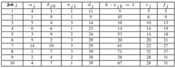
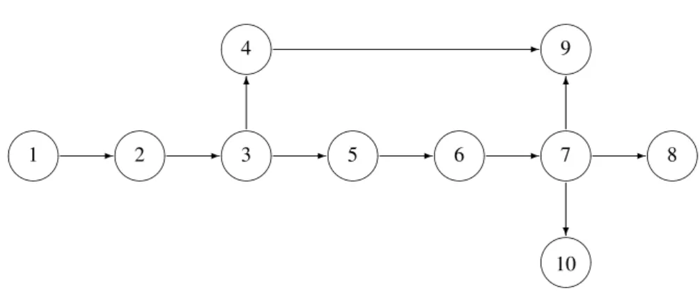
As a prelude, we present below an example to illustrate the problem under investigation and to gain insights into the proposed formulation. Consider the problem instance where the jobs to be processed are related via the prece-dence graph depicted in Figure 2 and where the associated parameters are provided in Table 1 (with the remaining data being generated as prescribed in Section 4.1). The available resources include a single CPU and one FPGA for poten-tial use. The discrete, time-indexed scheduling horizon has a projected length ofs= 39time-slots.
The solution produced by Model HWSW is summarized in Table 1, and is depicted in the Gantt-chart in Figure 3. This small-sized problem instance was solved to op-timality in 0.04 seconds. Observe that the slot values k for which xjk = 1, as specified in Table 1, indicate
in-directly when operations start their processing, as well as the processing components on which these operations are scheduled (by observing the time-slot ranges attributed to each software/hardware component). For instance, both jobs 9 and 10 start at the beginning of time-slot 28 and are completed at the end of time-slot 31. However, since x9,28 = x10,67 = 1, job 9 is scheduled on the CPU,
whereas job 10 is processed on FPGA 1.
Jobj αj δj0 πj1 dj k:xjk= 1 sj fj 1 4 1 1 11 5 5 5 2 1 9 1 9 45 6 9 3 5 4 3 14 10 10 13 4 0 6 1 23 14 14 19 5 3 9 2 24 53 14 18 6 5 2 3 29 20 20 21 7 14 10 3 29 61 22 27 8 1 7 3 39 71 32 37 9 2 4 2 38 28 28 31 10 4 7 1 39 67 28 31
Table 1: Data and results for an illustrative example
4.3
Computational results
Table 2 summarizes the results obtained for instances hav-ing n =10 and 20. The first column of this table spec-ifies the instance number as well as the number of jobs
and the maximum number of FPGAs involved. The sec-ond column provides the length of the scheduling hori-zon (number of time-slots). In the next three columns, we present the results obtained for solving the continuous or linear programming (LP) relaxation of Model HWSW, denoted HWSW, by allowing the x-variables to assume continuous values between 0 and 1. The optimal objective value of the continuous relaxation (ν(HWSW)), the ensu-ing computational time in seconds, and the % optimality gap, are reported for each instance. We define the % Gap
as= 100ν(HWSWν(HWSW)−ν(HWSW) ). The final two columns relate to solving Problem HWSW to optimality. Table 2 reveals that for these instances having up to 20 jobs, optimal solu-tions were obtained within manageable times.
Table 3 provides the results for the more challenging 30-job problem instances. Here, in addition to solving the problem to optimality, we demonstrate the effectiveness of employing two heuristics to derive good quality feasible solutions in a relatively timely fashion. In Table 3, in ad-dition to the LP solution, we report the first MIP solution produced by CPLEX during its branch-and-bound (B&B) exploration, as well the best available MIP solution that the solver could obtain within a specified computational limit of 300 CPU seconds. We compare these two heuristic ap-proaches to solving the problem to optimality by reporting the percentage deviation (% Dev.) between the heuristic solution value from the optimal solution value.
Whereas the LP relaxation objective values forn = 10
were triggered by the solver at every node explored in the B&B tree.
5
Conclusions
We have proposed a novel formulation for partitioning and scheduling precedence-related jobs on both hardware and software components over a time-indexed horizon. Our model effectively captures the nonpreemption assumption, the precedence constraints, the inviolable due-date restric-tions, and the processing times required over hardware and software components. Computational experience reported using randomly generated test instances reveals that opti-mal solutions can be computed (forn ≤20) within about 20 seconds. Forn = 30, we demonstrated the effective-ness of two branch-and-bound-based heuristic approaches in producing near-optimal solutions. In particular, using the branch-and-bound algorithm of CPLEX 10.1 to output the first MIP solution and the best MIP solution within a timelimit of 300 CPU seconds, the resulting heuristic solu-tions respectively sacrificed only 2% and 0.18% of optimal-ity on average, while achieving an average computational savings of 98.6% and 93.8%, respectively, as compared with determining optimal solutions. Thus, we recommend the use of such heuristic approaches for large instances in order to obtain near-optimal solutions with manageable ef-fort. Also, we have focused our attention on minimizing the total processing and resource costs. However, the proposed model is flexible enough to accommodate different alter-native objective functions of practical interest within this same modeling framework, which involve the makespan, resource usage (number of FPGAs, durations of usage of FPGAs, etc.), and the completion times of jobs, as desired.
Acknowledgement
This work has been partially supported by theNational Sci-ence Foundationunder Grant CMMI-0552676.
References
[1] Ali, F. M. and Das A. S. (2004), Hardware-software co-synthesis of hard real-time systems with reconfig-urable FPGAs, Computers and Electrical Engineer-ing, 471-489.
[2] Arato P., Juhasz S., Mann Z. A., Orban A. and Papp, D. (2003), Hardware-software partitioning in embed-ded system design,IEEE International Symposium on Intelligent Signal Processing, 197-202.
[3] Bender, A. (1996), Design of an optimal loosely cou-pled heterogeneous multiprocessor system, Proceed-ings of European Design and Test Conference, 275-281.
[4] Brogioli, M., Radosavljevic, P. and Cavallaro, J. R. (2006), A general hardware/software co-design methodology for embedded signal processing and multimedia workloads,Fortieth Asilomar Conference on Signals, Systems and Computers, 1486-1490. [5] Dasu, A. and Panchanathan, S. (2001),
Reconfig-urable media processing, Proceedings of Interna-tional Conference on Information Technology: Cod-ing and ComputCod-ing. 2-4 April 2001, 300 - 304. [6] Dittmann, F., Gotz, M. and Rettberg, A. (2007),
Model and methodology for the synthesis of hetero-geneous and partially reconfigurable systems, Par-allel and Distributed Processing Symposium, 2007, IPDPS 2007, IEEE International, 26-30 March 2007, 1-8.
[7] Edwards, M.D. and Forrest, J. (1995), Hard-ware/software partitioning for performance enhance-ment,IEEE Colloquium on Partitioning in Hardware-Software Codesigns, 2, 1-5.
[8] Fisher, M. L. (1976), A dual algorithm for the one ma-chine scheduling problem, Mathematical Program-ming, 11, 229-251.
[9] Giovanni, D.M. and Rajesh, K. G. (1997), Hard-ware/software co-design, Proceedings of the IEEE, 85(3), 349-365.
[10] Haubelt, C., Otto, S., Grabbe C. and Teich, J. (2005), A system-level approach to hardware reconfigurable systems,Proceedings of the Design Automation Con-ference ASP-DAC 2005, 298-301.
[11] Jeong, B., Yoo, S., Lee, S. and Choi, K. (2000), Hardware-software cosynthesis for run-time incre-mentally reconfigurable FPGAs, Proceedings of the Design Automation Conference ASP-DAC 2000, 169-174.
[12] Juan P. C., David, S., Onassis, C. and Al-varo, S. (2000), Pipelining-based tradeoffs for hard-ware/software codesign of multimedia systems, 8th Euromicro Workshop on Parallel and Distributed Processing, 383-390.
[13] Liu, H. and Wong, D. F. (1998), Integrated partition-ing and schedulpartition-ing for hardware/software co-design, Proceedings of the International Conference on Com-puter Design, 609-614.
[14] Niemann, R. and Marwedel, P. (1997), An algorithm for hardware/software partitioning using mixed inte-ger linear programming,Design Automation for Em-bedded Systems, 2(2), 165-193.
[16] Saul, J. M. (1999), Hardware/software codesign for FPGA-based systems, Proceedings of the 32nd An-nual Hawaii International Conference on System Sci-ences.
[17] Sherali, H. D. and Smith, J. C. (2001), Improving dis-crete model representations via symmetry considera-tions,Management Science, 47, 1396-1407.
[18] Shin, Y. and Choi, K. (1997), Enforcing schedulabil-ity of multi-task systems by hardware-software code-sign,International Workshop on Hardware/Software Co-Design, 3-7.
[19] Sipper, M. and Sanchez, E. (2000), Configurable chips meld software and hardware,IEEE Computer, 33(1), 120-121.
-1
-2
-3
6
4
6
9
?
10
-5
-6
-7
8
Figure 2: Task precedence graph for the illustrative example involving 10 tasks
CPU
FPGA 1
1 2 3 4 5 6 7 8 9 10 11 12 13 14 15 16 17 18 19 20 21 22 23 24 25 26 27 28 29 30 31 32 33 34 35 36 37 38 39 1
2
3
5
4 6
7 10 8
9
40 41 42 43 44 45 46 47 48 49 50 51 52 53 54 55 56 57 58 59 60 61 62 63 64 65 66 67 68 69 70 71 72 73 74 75 76 77 78
Figure 3: Gantt chart for an illustrative example involving 10 tasks and one FPGA
Instance s LP Solution MIP solution
#,(n, m) ν(HWSW) Time (s) % Gap ν(HWSW) Time (s)
1, (10,3) 42 387 0.05 1.5 393 0.35 2, (10,3) 69 413 0.09 0 413 0.09 3, (10,3) 59 363.8 0.11 1.6 370 0.20 4, (10,3) 71 431 0.12 0.2 432 0.14 5, (10,3) 62 396 0.09 0.2 397 0.12 6, (20,2) 40 639.66 0.12 20.2 803 0.39 7, (20,2) 44 649.30 0.11 22.4 838 1.45 8, (20,2) 58 829.14 0.14 23.0 1079 17.12 9, (20,2) 72 1008 0.10 22.2 1296 0.54 10, (20,2) 63 841 0.17 23.5 1100 20.93
Table 2: Performance of Model HWSW for instances havingn=10 and 20
Instance s LP Solution First MIP MIP within 300 s Optimal MIP
#,(n, m) ν(HWSW) Time (s) % Gap ν(HWSW) Time (s) % Dev. ν(HWSW) % Dev. ν(HWSW) Time (s)
11, (30,2) 77 1444.7 0.18 17.9 1769 6.3 0.4 1761 0 1761 10.8 12, (30,2) 74 1228.11 0.21 20.0 1571 17.4 2.2 1537 0 1537 103.93 13, (30,2) 57 1166.49 0.23 17.7 1484 21.6 4.5 1433 0.9 1419 6647.9 14, (30,2) 92 1175.98 0.39 19.2 1485 165.6 1.9 1466 ≈0 1456 2819.3 15, (30,2) 81 1639.24 0.39 9.6 1836 17.6 1.1 1815 0 1815 6943.7