Imprecise Computation Model,
Synchronous Periodic Real-time Task
Sets and Total Weighted Error
Damir Pole
s
ˇ
1and Leo Budin
21Eurocontrol Experimental Centre, Br´etigny sur Orge, France
2Faculty of Electrical Engineering and Computing, University of Zagreb, Croatia
This paper proposes two scheduling approaches, one-level and two-one-level scheduling, for synchronous periodic real-time task sets based on the Imprecise Computation Model. The imperative of real-time systems is a reaction on an event within a limited amount of time. Sometimes the available time and resources are not enough for the computations to complete within the deadlines, but still enough to produce approximate results. The Imprecise Computation Model is motivated by this idea, which gives the flexibility to trade off precision for timeliness. In this model a task is logically decomposed into a mandatory and optional subtask. Only the mandatory subtask is required to complete by its deadline, while the optional subtask may be left unfinished. Usually, different scheduling policies are used for the scheduling of mandatory and optional subtasks. For both proposed approaches the earliest deadline first and rate monotonic scheduling algorithms are used for the scheduling of mandatory subtasks, whereas the optional subtasks are scheduled in a way that the total weighted error is minimized. The basic idea of one-level scheduling is to extend the mandatory execution times, while in two-level scheduling the mandatory and optional subtasks are separately scheduled. The single preemptive processor model is assumed.
Keywords: Imprecise Computation Model,real-time sys-tems, one-level scheduling, two-level scheduling, total weighted error
1. Introduction
The correctness of many systems and devices in our society depends not only on the logical correctness of results they produce, but also on the time at which they are produced. These real-time systems play an important role and they have been included in the wide range of applications from nuclear power plants, rail-way systems, air traffic control, military and
health monitoring systems to telecommunica-tion networks, multimedia systems, monitor-ing systems, virtual realty and computer games. Since computers are more often used in our ev-eryday activities, real-time systems will be more important. Scheduling is concerned with the al-location of scarce resources and it is a central activity of a real-time system with the objective to meet specified time constraints. For some real-time systems, all specified timing require-ments must be met(hard real-time systems)and a failure to do so may lead to catastrophic con-sequences, whereas for others some specified timing requirements may be missed (soft real-time systems).
This paper presents the result of an analysis of the multi-level scheduling approach for dy-namic real time systems with flexible timing requirements. In particular, it proposes one and two-level scheduling approaches for the Impre-cise Computation Model. The imperative is to establish the theoretical lower bound for the to-tal weighted error for both approaches as the most complex error case. This directly leads to the lower bound for the total error and the upper bound for the processor utilization.
schedule in which all tasks meet timing and all other specified constrains.
Sometimes, it is not possible to create a feasible schedule, i.e. it is not possible for all tasks to meet their timing constraints. But, there still may be enough resources to produce approxi-mate results. The generation of partial results using less time and resources is the basis of Imprecise Computation Model. In the Impre-cise Computation Model ([3], [4], [6], [8], [9])
each task Ti is logically decomposed into two subtasks: mandatory subtask Mi and optional subtask Oi. Only the mandatory subtask of each task is required to be completed by the task’s deadline in order to produce a minimum quality, but still acceptable, result. The op-tional subtask does not have to be completed(if there is no available processor’s time). Simi-larly, a schedule is defined to be feasible in the Imprecise Computation Model when all manda-tory subtasks meet timing and all other specified constraints.
The task set used in the analysis consists of a set of nindependent, preemptable tasks, TS =
{T1,T2, . . . ,Tn}. TaskTiis characterized by the quintupleTi = (ri,di,mi,oi,pi)whereri,di,mi,
oi and pi denote the task’s ready time, relative deadline, mandatory subtask’s execution time, optional subtask’s execution time and the task’s period, respectively. The task’s total execution time is defined as ei = mi +oi. Appropriate mandatoryM and optionalOsubtask sets con-sist of n independent, preemtable tasks, M =
{M1,M2, . . . ,Mn}andO= {O1,O2, . . . ,On}. TaskMiis characterized by the quadrupleMi=
(ri,di,mi,pi) and Oi by Oi = (ri,di,oi,pi). Each task Ti, Mi and Oi generates an infi-nite number of jobs Tij, Mij, Oij, j > 0, with
rij = ri+ (j−1)pi and dij = di + (j−1)pi. The task set,TS, is assumed to be synchronous. A task set is said to be synchronous if all ready times are zeros, otherwise a task set is asyn-chronous. This implies that all ready times in our analysis are assumed to be equal to zero,
ri = 0. The tasks’ deadlines are assumed to be equal to tasks’ periods di = pi. Without loss of generality, integer values for all tasks’ parameters are assumed [1]. The synchronism of task set and integer parameters facilitate the analysis which, in this case, can be performed on the limited time period which is equal to hyperperiodH, the least common multiplier of all periods in TS, H = lcm(p1, . . . ,pn). The single preemptive processor system is assumed
and the context switching times are neglected. The processor utilization,U(TS), of task setTS
is defined asU(TS) = n
i=1
ei
pi.
2. Total Weighted Error
Since the Imprecise Computation Model gives the opportunity to trade-off between the result quality of computations and computation tim-ing requirements, a lot of different metrics have been introduced in order to validate the trade-off and set objectives. Accordingly, a lot of different definitions of errors that correspond to different measures, objectives and applications have been proposed in the literature, e.g. the total weighted error ([6], [4]), the normalized error [8], the maximum normalized error [8], the maximum weighted error[4], the fraction of discarded work [3], number of tardy tasks [6]. It is clear that the error which will be analyzed and objectives that will be optimized depend on an application. Further in this paper, only the total weighted error and its minimization is considered.
In general, the problem of minimizing the total weighted error may be transformed to the min-imizing the total weighted tardiness [2]or to a minimum-cost-maximum-flow problem[4]. In the paper, the total weighted error is analyzed for the synchronous periodic task sets with re-spect to the earliest deadline first(EDF)and rate monotonic (RM) scheduling algorithms used for scheduling of the mandatory subtask sets. LetSbe a feasible schedule for task setTS, and αij(Ti,S)denote the amount of processing time assigned for the execution of the jthjob of task
Tiin scheduleS. The amount of discarded work
[3], the error, of the jthjob of taskTiis defined to beε(Tij,S) = ei−αij(Ti,S). For synchronous periodic task setTSand feasible scheduleS, the error of taskTi in hyperperiod H is defined as follows:
ε(Ti,S,H) = ni
j=1
ε(Tij,S); ni= H
weighted error for task set TS and feasible scheduleSin hyperperiodHis defined as:
ε =ε(TS,S,H) =
n
i=1
wiε(Ti,S,H); (2)
where wi is the weight of error of task Ti. For task set TS it is assumedw1 ≥ . . . ≥ wn. The weight of error determinates the importance of the task. As the weight of error is higher the importance of the task is higher. In case of the total error, all weights are the same.
3. Scheduling
The scheduling of task setTSis based on the us-age of the EDF and RM scheduling algorithms for the scheduling of mandatory subtask set. It is assumed that the mandatory subtask set M
is schedulable by EDF and RM. Taking into account optional task set parameters, it is obvi-ous that the same scheduling algorithms for the optional subtask set at the same time or level cannot be applied.
Let a scheduling of Imprecise Computation Mo-del in which a scheduler is not able to consider the mandatory subtask set and the optional sub-task set separately, i.e. a scheduler applies the same scheduling policy for all tasks in a task set, be called one-level scheduling. On the other side, let a scheduling in which a sched-uler is able to consider the mandatory subtask set and the optional subtask set separately, i.e. a scheduler applies separate, possibly different, scheduling policies for mandatory and optional subtask sets, be called two-level scheduling. In the paper, both approaches are analyzed. In the first approach, the use of one-level schedul-ing is assumed. The idea is to extend manda-tory execution times of all mandamanda-tory subtasks in TS as much as possible in a way that the total weighted error of TS is minimized. The result of extension is task setMwhich consists of mandatory subtask set only and should be scheduled making use of EDF or RM.
In the second approach, the use of two-level scheduling is assumed and a scheduler must pro-duce schedules on two levels. On the high level the mandatory subtask set is scheduled while on the low level the optional subtask set is sched-uled. The high level has to ensure processor
time and its assignment to the low level. The low level has to ensure the execution of optional subtask set in a way that the total weighted error ofTSis minimized.
3.1. One-level scheduling
One-level scheduling approach is based on the creation of a new mandatory subtask setMthat extends mandatory execution times in compar-ison toM. The optional sub-task set,O, is not directly scheduled. It is included in the schedule of new mandatory sub-task set,M. The exten-sion of mandatory subtask set M is done in a way that the total weighted error is minimized. Finally, the schedulesS1andS2ofM, generated using EDF and RM, are used for scheduling task set TS. The extending process may be divided in the following steps:
• determination of the maximum extension,
extMAX, of mandatory execution times;
• determination of the extension for each man-datory subtaskMi,exti, in a way that the total weighted error is minimized.
The process starts fromMand results is the new task set M, M = {M1,M2, . . . ,Mn}, Mi = (ri,di,mi,pi), ri = 0, di = pi, mi = mi+exti, 0≤exti,∀i.
The maximum amount of time that can be as-signed for the extension of mandatory subtasks during hyperperiod H, extMAX, depends on a scheduling algorithm used. extMAX must ensure the schedulability ofM.
In the case of the EDF scheduling algorithm the maximum total extension time is defined as:
extMAX,EDF= (1−U(M))H, (3) whereU(M)is the utilization of mandatory sub-task setM. The value ofextMAX,EDFguarantees the utilization of M to be less or equal to 1,
U(M)≤1, which implies the schedulability of
M[5].
In the case of the RM scheduling algorithm, the maximum total extension time is defined as:
utilization of M to be less or equal to URM,n,
U(M) ≤ n(21/n−1) = U
RM,n, which implies the schedulability of M [5]. It is obvious that the sum of all extensions must be less or equal
toextMAX, regardless of the algorithm used:
n
i=1
niexti≤extMAX. (5)
The objective to minimize the total weighted er-ror ofTSin resulting scheduleSofMderives the conditions for the determination of manda-tory execution time extensions for all tasks, whether EDF or RM is used.
Taking into account thatε(Tij,S) =oi−exti,∀j from(1)and(2), we have:
ε(TS,S,H) =
n
i=1
winioi− n
i=1
winiexti (6)
whereniis the number of jobs of subtaskMi(or
Mi)occurred in hyperperiodH. The minimiza-tion of total weighted error implies the maxi-mization of the second member of the right side hand in(6):
min(ε(TS,S,H))⇒max n
i=1
winiexti. (7)
From(5)and(7), it follows that this problem of determination of extensions can be reduced to the bounded knapsack problem(BKP)for both scheduling algorithms, EDF and RM.
In BKP a knapsack with weight capacityband
nitems,j= 1, . . . ,n, with utility valuescj and weightsajis given. The quantities of items,xj, have to be calculated with limited total weight of the knapsack, b, and the upper bounds, bj, maximizing the value of the knapsack’s con-tent. BKP can be formulated as[2]:
max n
j=1
cjxj, subject to n
j=1
ajxj≤b, (8)
0≤xj ≤bj, j=1, . . . ,n, xjinteger. Assuming that all weights,aj, all utility values,
cj, and all upper bounds,bj, are positive integers,
the determination of extensions problem can be reduced to BKP with following parameters:
cj=wknk, aj =nk, xj =extk, bj=ok, (9)
b=extMAX, j=1, . . . ,n, k=1, . . . ,n, assuming that the tasks are reordered accord-ing to c1/a1 ≥ . . . ≥ cn/an. Since c1/a1 ≥
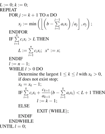
. . . ≥ cn/an implies w1 ≥ . . . ≥ wn, which is one of the assumptions, the reordering is not needed,j =k. This order is requested in order to apply a branch-and-bound algorithm, Algo-rithm 1, which is proposed for the calculation of an optimal solution of BKP problem. Al-gorithm 1 is a modified version of AlAl-gorithm Branch-and-Bound Knapsack for the knapsack problem, described in[2]. The modification is done in order to limit the extensions to optional execution times. In Figure 1 a detailed descrip-tion of Algorithm 1 is given.
L:=0;k:=0; REPEAT
FORj:=k+1 TOnDO
xj:=min
b−j−1 i=1aixi
/aj
,oj
; ENDFOR
IFn
i=1cixi>LTHEN
L:=n
i=1cixi; x ∗:=x;
ENDIF
l:=n−1; WHILEl>0 DO
Determine the largest 1≤k≤lwithxk>0,
if does not exist stop;
xk=xk−1;
IFk
i=1
cixi+ack+1 k+1(b−
k
i=1
aixi)<L+1 THEN
l:=k−1; ELSE
EXIT(WHILE); ENDIF
ENDWHILE UNTILl=0;
Figure 1.Algoritm 1.
The result of Algoritm 1 is an optimal so-lution, x∗, for BKP, i.e. a set of extensions
(ext1, . . . ,extn). For the EDF and RM schedul-ing algorithms the optimal solutions ( exten-sions) x∗EDF and x∗RM are generated using
extMAX,EDF and extMAX,RM, respectively. So-lutionsx∗EDFandx∗RMare used for the creation of
Mfor both scheduling algorithms(MEDF,MRM ).
3.2. Two-level scheduling
As mentioned, in this approach task set TS is scheduled on two levels. On the high level, mandatory subset M is scheduled and proces-sor time for optional subtask set O has to be ensured. This is done by adding a new manda-tory subtaskMn+1toMand as the result a new mandatory subtask set M is created. M must not harm the schedulability of M and the ex-ecution time of Mn+1 is assigned to optional subtask set O. The maximum possible execu-tion time for Mn+1 should be determined, the time intervals assigned to Mn+1 should be de-termined and optional subtask set Oshould be scheduled over found time intervals in a way that the total weighted error is minimized. This should be done for the EDF and RM scheduling algorithms.
Theorem 1. Let τ be a synchronous periodic task set, τ = {T1, . . . ,Tn}, Ti = (ri,di,ei,pi),
n,i ∈N, i ≤n,pi,ei ∈N, 1< p1 ≤. . . ≤ pn,
di = pi, ri = 0, schedulable by EDF and RM with the utilization less than 1,U(τ)<1. There exists synchronous periodic task setτ,τ =τ∪
{Tn+1};Tn+1 = (en+1,pn+1), which is schedu-lable by EDF and RM with the utilization equal to 1,U(τ) =1, wherepn
+1 =lcm(p1, . . . ,pn) anden+1= (1−U(τ))lcm(p1, . . . ,pn).
Proof: Let’s define task Tn+1 = (rn+1,dn+1,
en+1,pn+1), wherern+1=0,pn+1=H,dn+1 =
pn+1anden+1 = (1−U(τ))H. It is obvious that task set τ, τ = τ ∪ {Tn+1}, is a synchronous
periodic task set withU(τ) =1 and the
hyper-period equal to H, H = lcm(p1, . . . ,pn). Task set τexists with U(τ) = 1 and therefore it is
schedulable by EDF. LetSandSbe the sched-ules of task setsτandτproduced by RM. Both
schedules are repeated byH and it is sufficient to analyze the behaviour during H. TaskTn+1 has the lowest priority inτunder RM duringH.
The lowest priority of taskTn+1inτguarantees the same execution intervals of tasksT1, . . . ,Tn in S as inS during H. This implies that each of tasks T1, . . . ,Tn meets its deadline and that the idle intervals in S can be assigned for the execution of Tn+1 in S. The amount of time of all idle intervals in S is equal (1−U(τ))H
which is equal toen+1duringH. This confirms that taskTn+1meets its deadline and proves the schedulability of task setτunder RM.
According to Theorem 1 we have M = M ∪
{Mn+1}, rn+1 = 0, pn+1 = H, mn+1 = (1−
U(M))H, on+1 = 0, dn+1 = pn+1, where H is the hyperperiod ofM. Resulting subtask set
Mis schedulable by EDF and RM with the uti-lization equal to 1, i.e. the maximum possible execution time is assigned toMn+1.
In order to minimize the total weighted error the processor availability for mandatory subtask
Mn+1, has to be determined. Let’s define a busy period([1],[7])as an interval of time in which the processor is never idle. This implies that the processor availability for mandatory sub-task Mn+1, is equal to the idle periods of the schedule of mandatory subtask setM.
Theorem 2. LetS1andS2are feasible schedules for task set τ defined in Theorem 1 generated by the EDF and RM scheduling algorithms, re-spectively. Both schedules have the same busy periods.
Proof: Let’s assume thatS1andS2do not have the same busy periods andI, I = [t1,t2), be the first time interval during which an idle period is present in one schedule(Si) and a busy period in the other schedule(Sj). This implies that the amount of time assigned for the execution of the task set is the same inSi andSj untilt1. In
Si each started task’ job successfully finished its execution (i.e. all deadlines are met)by t1, while in Sj there is at least one ready job that has to finish its execution. There are two pos-sibilities inSjatt1: the execution of a task that just became ready at t1 and the execution of a task that became ready before t1. In the first case it is obvious that the task sets scheduled by Si and Sj are not the same, the task sets do not have the same periods. In the second case inSi all deadlines are met untilt1 while this is not the case forSj. Since the same amount of time is assigned to the task set execution in both schedules untilt1this implies that the execution times are not the same and, further, that the task sets scheduled by Si and Sj are not the same. This is against the hypothesis. If I is an idle period in one schedule it must be an idle period in another schedule.
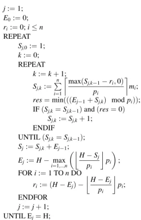
by EDF and RM Algorithm 2 is proposed. A detailed description of Algorithm 2 is given in Figure 2.
j:=1;
E0:=0;
ri:=0;i≤n
REPEAT
Sj,0:=1;
k:=0; REPEAT
k:=k+1;
Sj,k:= n
i=1
max(Sj,k−1−ri,0)
pi mi;
res=min(((Ej−1+Sj,k) modpi));
IF(Sj,k=Sj,k−1)and(res=0)
Sj,k:=Sj,k+1;
ENDIF
UNTIL(Sj,k=Sj,k−1);
Sj:=Sj,k+Ej−1;
Ej:=H− max i=1,..,n
H−Sj
pi
pi
; FORi:=1 TOnDO
ri:= (H−Ej)−
H−Ej
pi
pi;
ENDFOR
j:=j+1; UNTIL Ej=H;
Figure 2.Algorithm 2, an iterative algorithm for finding the idle intervals.
As the result of applying Algorithm 2 onM, the available time intervals for scheduling optional subtask O are provided, TI = {[S1,E1), . . . ,
[Sl,El)}, l ∈ N. Note that precedence con-straints between the mandatory and optional subtasks are already included in TI, i.e. there is no need for ready optional tasks to wait with the execution.
Finally, optional subtask setOshould be sched-uled minimizing the total weighted error of task set TS. This is done by making use of Al-gorithm WNTU [4]. Algorithm WNTU mini-mizes the total weighted error. It was devel-oped for an aperiodic task set which implies that the optional subtask setOneeds to be trans-lated into aperiodic task setATSover observed time interval, H. This is done by consider-ing each task’s job as a separate task over H. As the result we have aperiodic task setATS=
{O1,1, . . . ,O1,n1,O2,1, . . . ,O2,n2, . . . ,On,1, . . . ,
On,nn}, Oi,j is the task that corresponds to the jth job of the ith subtask; Oij(rij,dij,eij), rij =
(j−1)pi, dij = jpi, eij = oij, ni = H
pi. WNTU algorithm supposes different weights, i.e.w1 >
· · · > wk. If task setATS contains more than
one task with the same weight, the grouping is needed. All tasks with the same weights form a subset of tasks with the same weights. There areksubsets(k≤n)each of which contains all jobs of the tasks with the same weight. LetTSSi be a subset which contains all tasks with weight
wi and Vj the jth busy period block. In addi-tion, letSCbe an empty schedule andET be an empty set. A detailed description of Algorithm WNTU is given in Figure 3.
SC=∅,ET=∅; FORj:=1 TOkDO
SCj:=Algorithm NTU forET∪TSSj;
Begin(Adjustment Step)
Let there beqblocks inSC: Vi= [vi−1,vi],
1≤i≤q. FOR i :=1 TO q DO
IFViis a task block inSC, THEN
Let tasklbe executed withinViinSC.
LetN(l) (resp.Nj(l))be the number of
time units joblhas executed inSC(resp.
SCj)from the beginning until timevi.
IFN(l)>Nj(l), THEN
assign (N(l)−Nj(l)) more time
units to task lwithinViinSCj, by
replacing any task, except task l, that was originally assigned within
Vi.
ENDIF ENDIF ENDFOR End
SC
j :=SCj.
Set the execution time of each task in TSSjto be the
number of nontardy units inSC j.
ET :=ET∪TSSj
SC:=Algorithm NTU forET. ENDFOR
Figure 3.Algorithm WNTU.
[Sj,Ej). A detailed description of Algorithm NTU is given in Figure 4. l is the number of idle periods and mis the number of tasks to be scheduled.
li:=Ei−Si;i≤l
FORi=1, . . . ,mDO Find min(p)|Sp>ri;
Find max(q)|Eq≤di;
IFp≤q
FORj=q, . . . ,pDO
δ :=min(lj,ei);
SM(i,j):=δ;lj:=lj−δ;ei:=ei−δ;
ENDFOR ENDIF ENDFOR
Figure 4.Modified Algorithm NTU.
At the end of Algorithm WNTU, the schedule of subtask set O which minimizes the total weighted error ofTSis provided. This schedule is used together with schedules ofMgenerated by EDF and RM.
4. Conclusion
In this paper, the analysis of Imprecise Compu-tation Model for synchronous periodic task sets is provided. The analysis is based on the use of the EDF and RM scheduling algorithms for the mandatory subtask sets and the minimization of total weighted error. The scheduling of the optional subtask set is affected by the minimiza-tion of total weighted error. Two different ap-proaches are proposed, one-level and two-level scheduling approach. The results are the opti-mal schedules with respect to the total weighted error, whether the EDF or RM scheduling algo-rithm is used for the scheduling of mandatory subtask set.
In one-level scheduling approach, the manda-tory subtask set is transformed into the new mandatory subtask set extending the mandatory execution times as much as possible in order to minimize the total weighted error. The schedul-ing is done for the new mandatory subtask set instead of the original task set on one level us-ing EDF and RM. This approach has simpler implementation, but the flexibility of Imprecise Computation Model is lost. The lower total weighted error is achieved for the EDF schedul-ing algorithm because of its higher least upper
bound to processor utilization with respect to RM.
For two-level scheduling, the scheduling of man-datory subtask set is done on one level using EDF and RM while the scheduling of optional subtask set is done on a separate level minimiz-ing the total weighted error. This approach has more complex implementation, but the flexibil-ity is kept and the time isolation between the mandatory and the optional sets is obtained. The same total weighted error is achieved for the EDF and RM scheduling algorithms because they generate same idle intervals.
In comparison with two-level scheduling, a lo-wer total weighted error is expected for one-level scheduling due to the uniform distribution of job extensions. An interesting application case is the minimization of total error where the weight of error of each task is the same. The result is the maximum processor utilization for the given task sets.
The lowest total weighted error boundary for both scheduling approaches is established, but there are still a lot of different, open questions such as the comparison of two different schedul-ing approaches, the time complexity, the im-provements of existing algorithms, the usage of new algorithms and possible application areas. The findings in the paper are expected to be the theoretical basis for all open questions and improvements in the future.
References
[1] S. BARUAH, R. HOWELL, L. ROSIER, Algorithms and Complexity Concerning the Preemptive Scheduling of Periodic, Real-Time Tasks on One Processor.
Real-Time Systems, 2(1990), pp. 301–324.
[2] P. BRUCKER, S. KNUST,Complex Scheduling, Berlin Heidelberg: Springer-Verlag; 2006.
[3] W. FENG, J. W. S. LIU, Algorithms for Scheduling Real-Time Tasks with Input Error and End-to-End Deadline.IEEE Transactions on Software Engineer-ing, 23(2) (1997), pp. 93–106.
[4] J. Y-T. LEUNG, Imprecise Computation Model:
To-tal Weighted Error and Maximum. In Handbook of Real-Time and Embedded Systems (I. Lee, J. Y-T. Leung, S. H. Son, Ed.),(2008)pp. 7-1–7-14. Chapman & Hall/CRC.
[5] C. LIU, J. LAYLAND, Scheduling algorithms for
multiprogramming in a hard-real-time environment.
[6] J. W. S. LIU, K. J. LIN, W. K. SHIH, A. C. YU, J.
Y. CHUNG, W. ZHAO, Algorithms for Scheduling Imprecise Computation.IEEE Computer, 5(1991), pp. 58–68.
[7] R. PELLIZZONI, G. LIPARI, Feasibility Analysis of
Real-Time Periodic Tasks with Offsets.Real-Time Systems, 30(2005), pp. 105–128.
[8] W. K. SHIH, J. W. S. LIU, Algorithms for Scheduling
Imprecise Computations with Timing Constraints to Minimize Maximum Error. IEEE Transactions on Computers, 44(3) (1995), pp. 466–471.
[9] J. W. S. LIU, K. J. LIN, W. K. SHIH, A. C. YU, J. Y.
CHUNG, W. ZHAO, Algorithms for Scheduling
Im-precise Computations. InFoundations of Real-Time Computing: Scheduling and Resource Management (A. M. Van Tilborg, G. M. Koob, Ed.),(1991)pp. 203–249. Norwell, Kluwer Academic Publishers.
Received:June, 2010
Accepted: November, 2010
Contact addresses:
Damir Poles Eurocontrol Experimental Centre Centre de Bois des Bordes BP 15 F-91222 Br´etigny sur Orge France e-mail:[email protected]
Leo Budin Faculty of Electrical Engineering and Computing Unska 3 HR-10000 Zagreb Croatia e-mail:[email protected]
DAMIRPOLESˇholds Dipl. Ing. degree in electrical engineering from the Faculty of Electrical Engineering and Computing, University of Zagreb and M.Sc. degree in technical science, Interdisciplinary Postgraduate Study “Guidance and Control of Moving Objects”, University of Za-greb. He is a Ph.D. student at the Faculty of Electrical Engineering and Computing, University of Zagreb and he works for the Eurocontrol Experimental Centre as a senior assistant in aircraft performance mod-elling. His professional interests include real-time systems, modelling and simulations and software engineering.