Consistent cotrending rank selection when both stochastic and. nonlinear deterministic trends are present

(1)

Consistent cotrending rank selection when both stochastic and

nonlinear deterministic trends are present

Zheng-Feng Guo and Mototsugu Shintani y

This version: April 2010

Abstract

This paper proposes a model-free cotrending rank selection procedure based on the eigenstructure of a multivariate version of the von Neumann ratio, in the presence of both stochastic and nonlinear deterministic trends. Our selection criteria are easily implemented and the consistency of the rank estimator is established under very general conditions. Simulation results suggest good …nite sample properties of the new rank selection criteria. The proposed method is then illustrated through an ap-plication of Japanese money demand function allowing for the cotrending relationship among money, income and interest rates.

Department of Economics, Vanderbilt University, VU Station B #351819, Nashville, TN 37235-1819. Email:

[email protected]

y_{Department of Economics, Vanderbilt University, VU Station B #351819, Nashville, TN 37235-1819.} _Email:

(2)

1 Introduction

For decades, one of the most important issues in the analysis of macroeconomic time series has been how to incorporate a trend. Two popular approaches that have been often employed in the literature are (i) to consider a stochastic trend (with or without a linear deterministic trend), such as the one suggested in Nelson and Plosser (1982) and (ii) to consider a nonlinear deterministic trend such as the one with trend breaks considered in Perron (1989, 1997). Cointegration, introduced by Engle and Granger (1987), is a useful concept in understanding the nature of comovement among variables based on the …rst approach. In cointegration analysis, the cointegrating rank, de…ned as the number of linearly independent cointegrating vectors, provides valuable information regarding the trending structure of a multivariate system with stochastic trends. Several model-free consistent cointegrating rank selection procedures have been developed in the literature. Analogous to cointegration analysis, we can also investigate the nature of comovement based on the second approach, namely the nonlinear deterministic trend. The cotrending analyses of Bierens (2000), Hatanaka (2000) and Hatanaka and Yamada (2003) are along this line of research. However, the consistent selection procedure of the cotrending rank, de…ned similarly as the cointegrating rank with a stochastic trend replaced by a nonlinear deterministic trend, has not yet been developed.

This paper proposes a model-free consistent cotrending rank selection procedure when both stochastic and nonlinear deterministic trends are present in a multivariate system. Consistency here refers to the property that the probability of selecting the wrong cotrending rank approaches zero as sample size tends to in…nity. Our procedure selects the cotrending rank by minimizing the von Neumann criterion, similar to the one used by Shintani (2001) and Harris and Poskitt (2004) in their analyses of cointegration. This approach exploits the fact that identi…cation of cotrending rank can be interpreted as identi…cation among three groups of eigenvalues of the generalized von Neumann ratio. Using this property of the von Neumann criterion, we propose two types of cotrending rank selection procedures that are (1) invariant

(3)

to linear transformation of data; (2) robust to misspeci…cation of the model; and (3) valid not only with a break in the trend function but also with a certain class of a smooth nonlinear trend function. The simulation results also suggest that our cotrending rank procedures perform well in the …nite sample.

Our analysis is closely related to Harris and Poskitt (2004) and Cheng and Phillips (2009), who propose consistent cointegrating rank procedures that do not require a parametric vector autoregressive model of cointegration such as the one in Johansen (1991). While we mainly discuss a class of smooth transition trend models as our preferred speci…cation of the nonlinear trend function, our cotrending rank procedure does not rely on the parametric speci…cation of the trend function, nor the parametric speci…cation of serial dependence structure. Thus, our approach is more general than that of Harris and Poskitt (2004) and Cheng and Phillips (2009) in the sense it allows both common stochastic trends and common deterministic trends. Consequently, we can use the procedure to determine the cointegrating rank in the absence of nonlinear deterministic trends. To illustrate this ‡exibility, we also provide the simulation results to evaluate the performance of our procedure when it is applied to cointegrating rank selection.

As emphasized in Stock and Watson (1988), the cointegrated system can be interpreted as a factor model with a stochastic trend being a common factor. Thus, determining the cointegrating rank is identical to determining the number of common stochastic trends because the latter is the di¤erence between the dimension of the system (number of variables) and the cointegrating rank.1 In the presence of both stochastic and nonlinear deterministic trends, however, the number of common nonlinear deter-ministic trends does not correspond to the di¤erence between the dimension and the cotrending rank. Because the number of common deterministic trends also contains valuable information on the trending structure, we introduce the notion of weak cotrending rank so that the di¤erence between the dimension and the weak cotrending rank becomes the number of common deterministic trends. Our procedure can

1

PANIC method proposed by Bai and Ng (2004) utilizes the consistent selection of the number of common stochastic trends in a very large dynamic factor system based on information criteria. See also Bai and Ng (2002) for the case of consistent selection of the number of stationary common factors.

(4)

select both a cotrending rank and a weak cotrending rank.

Our cotrending notion can be interpreted as a type of a common feature discussed in Engle and Kozicki (1993). They de…ne the common feature as “a feature that is present in each of a group of series but there exists a non-zero linear combination of the series that does not have the feature”. Our de…nition of cotrending also requires a non-zero linear combination to eliminate nonlinear deterministic trends. Our cotrending analysis is also related to cobreaking analysis of Hendry and Mizon (1998) and Clements and Hendry (1999). In the presence of a trend break, cobreaking is a necessary condition of cotrending but not a su¢ cient condition.

The remainder of this paper is organized as follows. Section 2 introduces several techniques to model deterministic trends and some key concepts in the presence of stochastic and deterministic trends. The main theoretical results are given in section 3. Section 4 reports Monte-Carlo simulation results to show the …nite sample performance of our procedures. In section 5, we apply our procedures to the Japanese money demand function. Section 6 concludes and the technical proofs are presented in the Appendix.

2 Motivation

2.1 A smooth transition trend model

The traditional approach to introduce a deterministic trend in a scalar time series_fytgTt=1 is to consider

a simple linear trend model given by

yt=dLINt +"t

and

(5)

wheredLIN_t is a linear trend function and"tis a zero-mean stationary error component. Serial correlation

is typically allowed in the error term, but we focus on the case of i.i.d. white noise to simplify the argument. Using this linear trend model to …tyt, measured in logarithms, is appropriate when the (log)

growth rate of the variable is stable over the sample period around the average (log) growth rate of . However, as discussed in Mills (2003), many macroeconomic time series data, including GDP of the UK and Japan, and stock prices in the U.S., violated the assumption of stable growth over the sample.

A convenient approach to allow for multiple shifts in the average growth rate while maintaining the continuity of the trend function is to consider a kinked trend, or a piece-wise linear trend structure in each segment of the whole sample period. When there are h time shifts in the average growth rate, a

segmented linear trend model can be de…ned as

yt = dKIN Kt +"t;

dKIN K_t = c+ ₀t+

h

X

i=1

i(t Ti)1[t > Ti];

wheredKIN K_t is a piece-wise linear trend function,Ti is the break point, and 1[x]is an indicator which

takes the value of 1 ifxis true and 0 otherwise. The segmented linear trend model above implies that the

average growth rate during the …rst subperiodt < T1 corresponds to 0, and the remaining subperiods,

Tj t < Tj+1 for j = 1; :::; h corresponds to 0 +

Pj

i=1 i. As long as the break point is known, the

model can be estimated using the least squares estimator.

Although the segmented trend functiondKIN K_t imposes continuity, its …rst derivative is not

continu-ous, suggesting an abrupt change of the growth rate at each break point. To allow for a gradual change in the growth rate, we may replace the indicator function in dKIN K

t with a smooth transition function.

This substitution of the trend function leads to a smooth transition trend model. The smooth transition trend model was originally proposed by Bacon and Watt (1971) and has been discussed by Granger and

(6)

Teräsvirta (1993), Teräsvirta (1994) and Greenaway, Leybourne and Sapsford (1997). While there are many types of smooth transition trend functions, the most frequently used one is the logistic transition function given by

G( _i; Ti) =

1

1 + exp( _i(t Ti))

;

where _i is the scaling parameter which controls the speed of transition, and Ti becomes the timing of

the transition midpoint instead of the break point.

A multiple-regime logistic smooth transition trend (LSTT) model takes the form of

yt = dLSTt +"t;

dLST_t = c+ ₀t+

h

X

i=1

i(t Ti)G( i; Ti)

wheredLST

t is the nonlinear linear trend function which we mainly focus on in our cotrending analysis.

It should be noted that as _i approaches in…nity, the logistic transition function G( _i; Ti) approaches

the indicator function1[t > Ti]. Thus, our deterministic trenddLSTt nests both the kinked trenddKIN Kt

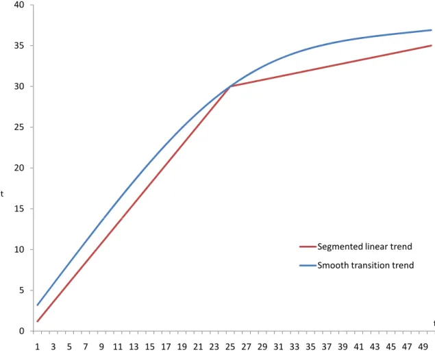
and the linear trend dLIN

t as a special case. Figure 2.1 shows the typical shape of kinked and smooth

transition trends whenh= 1. The former contains a one-time abrupt change in the …rst derivative while

the latter shows continuous change in the …rst derivative.

2.2 Cointegration and common deterministic trend

(1) Stochastic trends only

Cointegration, a very important concept in trending analysis of macroeconomic time series, was …rst introduced by Engle and Granger (1987). Multivariate integrated processes of order one are cointegrated if some linear combination of the same series becomes stationary. For example, suppose that a pair of

(7)

variables yt= (y1t; y2t)0 are generated from two random walk processes as in

y1t = s1t; y2t=s2t;

s1t = s1t 1+"1t; and

s2t = s2t 1+"2t:

Since there is no linear combination ofy1tandy2tthat yields stationarity,ytis not cointegrated. Instead,

suppose that the pair are generated from one random walk component as in

y1t = s1t; y2t=s2t;

s1t = s1t 1+"1t and

s2t = s1t+"2t:

Since y1t y2t = "2t is stationary,yt is cointegrated with a cointegrating vector (1; 1). This simple

example shows that cointegration requires the pair to share a common stochastic trend s1t.

(2) Deterministic trends only

Let us now turn to the case of deterministic trends. We refer cotrending among the variables with deterministic trends to the case when variables share a common deterministic trend. Suppose that each variable in the pairyt= (y1t; y2t)0 is generated from the linear trend model as in

y1t=dLIN1t ; y2t=dLIN2t

where dLIN

1t and dLIN2t are linear trend functions with potentially di¤erent intercepts and trend slope

coe¢ cients. Unlike the preceding example, we can always …nd the linear combination that eliminates the trend function (namely, the linear combination becomes a constant). Thus, the notion of cotrending in

(8)

the case of a linear trend is trivial. However, if the linear trend functions,dLIN₁_t and dLIN₂_t , are replaced with segmented trend functions, dKIN K₁_t and dKIN K₂_t , we can eliminate the deterministic trend if and only if (i) all of the break points,Ti’s, are the same (common break) and (ii) all of the piece-wise trend

slope coe¢ cients _iare proportional between the two trend functions. If either of the two conditions fails to hold, the two nonlinear deterministic trends are linearly independent and no common deterministic trend exists. A similar arguments apply when the segmented linear trends are replaced with smooth transition trends.

(3) Both stochastic and deterministic trends

When variables contain both stochastic and deterministic trends, there will be a layer of potential cotrending relationships. Suppose that a pair of variables,yt= (y1t; y2t)0, are generated from two random

walk with a drift processes as in

y1t = 1+y1t 1+"1t;

y2t = 2+y2t 1+"2t;

where ₁ ₆= 0 and ₂ ₆= 0. Then, the model can be rewritten as

y1t=dLIN1t +s1t; y2t=dLIN2t +s2t;

where

dLIN₁_t = s10+ 1t; dLIN2t =s20+ 2t;

(9)

In this case, the vector(1; ₁= ₂) eliminates the linear deterministic trend but does not eliminate the stochastic trend. In contrast, if the pair is generated from

y1t=dLIN1t +s1t; y2t=dLIN2t +s2t;

where

dLIN₁_t = s10+ 1t; dLIN2t =s20+ 2t;

s2t = s1t+"2t;

the vector(1; 1)eliminates the stochastic trend, and the vector(1; ₁= ₂)eliminates the linear deter-ministic trend. Therefore, the vector (1; 1) cannot eliminate both stochastic and deterministic trends

except for the case when ₁ = ₂. For the purpose of distinguishing between these two possibilities, Ogaki and Park (1997) introduce the notions of stochastic cointegration and deterministic cointegration. Stochastic cointegration refers to the case in which only the stochastic trend is eliminated while deter-ministic cointegration refers to the case in which both stochastic and deterdeter-ministic trends are eliminated at the same time.

While Ogaki and Park (1997) do not consider more general nonlinear deterministic trends, similar concepts can also be used when the linear trends, dLIN₁_t and dLIN₂_t , are replaced by either segmented trends, dKIN K₁_t and dKIN K₂_t , or smooth transition trends, dLST₁_t anddLST₂_t . In our analysis of cotrending, we are interested in the case of deterministic cointegration when the nonlinear deterministic trends are represented by a class of smooth transition trend models (which includes linear and kinked trends). To be more speci…c, we identify the total number of linearly independent vectors that can eliminate both stochastic and nonlinear deterministic trends. In this paper, we refer to the number of such cotrending

(10)

vectors as the cotrending rank and denote it byr1. In a system ofm variables with both stochastic and

deterministic trends, the cotrending rank can be any integer value in the range of 0 r1 < m. When

no variable contains deterministic trends, our de…nition of cotrending rank corresponds to that of usual cointegrating rank.

In addition to the cotrending rank, we also consider the total number of linearly independent vectors that can eliminate the deterministic trend regardless of whether such vectors can eliminate the stochastic trend at the same time. In the above example, a vector(1; ₁= ₂)can eliminate the deterministic trend regardless of the values of ₁ and ₂. We refer to this number as the weak cotrending rank and denote it by r2. Since all the cotrending vectors are also included in the weak cotrending vector, r2 should

satisfyr1 r2 < m. While it is not a cotrending rank, identi…cation of r2 is important sincem r2 in

them-variable-system with both stochastic and deterministic trends corresponds to the total number of

common deterministic trends.

In the next section, we propose a simple procedure to identify both r1 and r2 in a system of m

variables, in the presence of both stochastic and deterministic trends.

3 Theory

We assume that an m-variate time series,yt= [y1t; ; ymt]0, is generated by

yt=dt+st; t= 1; T; (1)

wheredt= [d1t; ; dmt]0 is a nonstochastic trend component,st= [s1t; ; smt]0 is a stochastic process,

respectively de…ned below, and neitherdtnorstare observable. We denote a random (scalar) sequencexT

byOp(T ) ifT xT is bounded in probability and byop(T )ifT xT converges to zero in probability.

(11)

respectively. The …rst di¤erence ofxt is denoted by xt. Below, we employ a set of assumptions that

are similar to the ones in Hatanaka and Yamada (2003).

Assumption 1. (i) st =st 1+ t and t =C(L)"t =P1j=0Cj"t j; C0 =In , P1j=0j2kCjk<1,

where"tisiidwith zero mean and covariance matrix "">0:(ii) Each element ofPT_t₌₁dtisO(T2)and

is not o(T2₎_:_{(iii) There exists an} _m _m _{orthogonal full rank matrix} _B _{= [}_B

? B2 B1 ] such that each

element ofPT_t₌₁B₁0ytisOp(T1=2), each element ofPTt=1B

0

2ytisOp(T)and is notop(T), and each element

of PT_t₌₁B_?0 yt isOp(T2) is not op(T2), where B1, B2; B_? are m r1,m (r2 r1) and m (m r2),

respectively.

Under Assumption 1, B1 represents a set of cotrending vectors which eliminates both deterministic

and stochastic trends. B2 represents a set of vectors which eliminates only deterministic trends, but not

stochastic trends. B_? consists of vectors orthogonal toB1 and B2.

In scalar case, the von Neumann ratio is de…ned as the sample variances of the di¤erences and the level of a time series. The multivariate generalization of the von Neumann ratio is de…ned as S₁₁1S00

where

S11=T 1

T

X

t=1

yty

0

t; and S00=T 1

T

X

t=2

yt y

0

t:

Shintani (2001) and Harris and Poskitt (2004) also use this multivariate version of the von Neumann ratio in cointegration analysis. Let b1 b2 bm 0be the eigenvalues ofS111S00. We summarize the

statistical properties of b0_is in the presence of both stochastic and deterministic trends in the following lemma.

Lemma 1 Under Assumption 1, we have: (i) a sequence of [b1, , br1] has a positive limit and is Op(1) but is not op(1); (ii) a sequence of T[br1+1, , br2] has a positive limit and is Op(1) but is not op(1), provided r2 r1 >0; and (iii) a sequence of T2[br2+1, , bm] has a positive limit and isOp(1)

(12)

but is not op(1), providedm r2 >0.

From Lemma 1, the eigenvalues of S₁₁1S00 can be classi…ed into three groups depending on their

rates of convergence, namely, Op(1) , Op(T 1) , and Op(T 2). The number of eigenvalues in each

group corresponds to the number of cotrending relationships, the di¤erence between weak cotrending and (strict) cotrending relationships, and the number of common deterministic trends, respectively. We exploit this property to construct the following two types of consistent cotrending rank selection procedures based on the von Neumann criterion de…ned as a sum of the partial sum of eigenvalues and a penalty term. The …rst is a paired procedure which independently selects the cotrending rank r1 and

the weak cotrending rank r2 by minimizing each of

V N1(r1) =

r1 X

i=1

b_i+f(r1)

CT

T ; and

V N2(r2) =

r2 X

i=1

b_i+f(r2)

C_T0 T2;

or

b

r1 = arg min 0 r1 m

V N1(r1); and

b

r2 = arg min 0 r2 m

V N2(r2)

wheref(r),CT and C

0

T are elements of penalty function de…ned in detail below.

Alternatively, we can simultaneously determine both r1 and r2 by minimizing

V N(r1; r2) =

p T r1 X i=1 b_i r2 X

i=r1+1

b_i+f(r1)

CT

T +f(r2) C_T0 T2;

(13)

or

(br1;rb2) = arg min 0 r1;r2 m

V N(r1; r2):

The main theoretical result is provided in the following proposition.

Proposition 1 (i) Suppose Assumption 1 holds, f(r) is an increasing function of r, CT; C

0

T ! 1,

CT=T; C_T0 =T;!0, then the paired procedure using V N1(r1) and V N2(r2) yields,

lim

T!1P(rb1=r1;rb2=r2) = 1: (ii) Suppose Assumption 1 holds,f(r)is an increasing function ofr,CT=

p

T ; C_T0 =pT _{! 1},CT=T; C_T0=T;!

0, then the joint procedure using V N(r1; r2) yields,

lim

T!1P(rb1=r1;rb2=r2) = 1: Remarks:

(a) The above proposition implies that both of the two cotrending rank selection procedures are consistent in selecting cotrending rank without specifying a parametric model.

(b) The criterion functionV N1(r1) in the paired procedure, can be used to select cointegrating rank

in a system with only a stochastic trend. It nests the criterion function considered in Harris and Poskitt (2004) as a special case. In contrast, the information criteria for selecting cointegrating rank in Cheng and Phillips (2009) are based on the eigenstructure of reduced rank regression model.

(c) A popular choice ofCT andC

0

T, in the literature of information criteria includesln(T);ln(ln(T)),

or2, which respectively leads to BIC, HQ, and AIC. The proposition implies that our cotrending rank

(14)

In the simulations, we also consider C_T0 = ln(T) ln(T) which yields consistency.

(d) For consistency, f(r) can be any increasing function of r. In this paper, we considerfHP(r) =

2r(2m+r 1)from Harris and Poskitt (2004) andfCP(r) =r(2m+ (r+ 1)=2)discussed in the footnote

1 of Cheng and Phillips (2009).

(e) Provided CT = CT0 , the pair of selected cotrending ranks obtained from the paired procedure

satis…esr_b1 br2.

(f) In the absence of deterministic trend with m = 1, r1 = 0 corresponds to a unit root case and

r2 = 1 corresponds to the stationary case.

4 Experimental evidence

4.1 Stochastic trend and cointegration

The selection procedures developed in the previous section are based on asymptotic theory. It is of interest to examine their …nite sample properties by means of Monte Carlo analysis. For this purpose, this section reports the results under di¤erent settings of the true cotrending ranks, and of various penalty terms.

As noted in the previous section, our procedures are more general than that of Harris and Poskitt (2004) and Cheng and Phillips (2009), and the criterion function V N1(r1) in the paired procedure can

also determine the cointegrating rank in the absence of nonlinear deterministic trend. In this subsection, the …nite sample performance ofV N1(r1)is evaluated and compared to the performance of cointegrating

rank selection procedures proposed by Harris and Poskitt (2004) and Cheng and Phillips (2009). We follow Cheng and Phillips (2009) and generate a bivariate time series yt= (y1t; y2t)0 using

yt=

0

(15)

where ut follows a V AR(1) process with VAR coe¢ cient0:4 I2 with mutually independent standard

normal error term. By setting 0 = 0,

0

= 1

0:5 ( 1 1 );

and

0

= 0:5 0:1 0:2 0:15 ;

we generate a multivariate system with the true cointegrating rank being 0;1 and 2, respectively. We

generate the data for two sample sizes T = 100 and T = 400. To eliminate the e¤ect of the initial

values y0 = 0 and u0 = 0; the …rst 100 observations are discarded. We evaluate the performance of

the procedures based on the frequencies of selecting the true cointegrating rank in 20,000 replications. For the reduced rank regression procedure of Cheng and Phillips (2009), we employ the AIC, BIC and HQ criteria and denote them by RRR-AIC, RRR-BIC and RRR-HQ, respectively. ForV N1(r1), we use

fHP(r) = 2r(2m r+ 1) as in Harris and Poskitt (2004), and CT = 2; log(T), and log(log(T)), and

denote corresponding criteria by ,VN-AIC, VN-BIC, and VN-HQ, respectively. The consistent selection criterion of Harris and Poskitt (2004) ( C;T in their notation) is identical to our VN-BIC. It should also

be noted that both RRR-AIC and VN-AIC are inconsistent in selecting true cointegrating rank. Table 1 reports the performance of the cointegrating rank selection procedures based on six criteria with the frequencies of correctly selecting true rank denoted in bold type. Among the procedures based on the von Neumann criterion, when sample size is large, VN-BIC outperforms other procedures. The good performance of BIC-based criterion is consistent with the similar …nding by Cheng and Phillips (2009) who compare the performance among reduced rank regregssion-based procedures. On the whole, the performance of the procedure based on the von Neumann criterion is comparable to that of Cheng

(16)

and Phillips (2009) in selecting cointegrating rank.2

4.2 Stochastic and deterministic trends and cotrending

In this section, we conduct a Monte Carlo experiment to investigate the …nite sample performance of our proposed cotrending rank selection procedure. We consider a three-dimensional vector series

yt = (y1t; y2t; y3t)0 with di¤erent combinations of cotrending and weak cotrending ranks. First, we

generate using

y1t = 1y1t 1+"1t;

y2t = 2y2t 1+"2t;

y3t =

c+ ₀t ift T

c+ ( ₀ ₁) T+ ₁t ift > T ;

with("1t; "2t)0 =iidN(0; ") where

"=

1 0:5 0:5 1 :

By using di¤erent combinations of _i _{2 f}0:5;1:0_gfori= 1;2, we control cotrending and weak cotrending ranks. We generate the data with (r1; r2) = (0;2), (1;1), and (2;0). The parameters for the kinked

trend function are set to c= 0:5, ₀ = 2, = 0:5;and ₁= 0:5. Second, we generate the data using

y1t = 1y1t 1+"1t;

y2t = 2y2t 1+"2t;

y3t = 3y3t 1+"3t;

2

While not reported, similar results are obtained for the case of di¤erent simulation design using other serial correlation structure foru.

(17)

with("1t; "2t; "3t)0 =iidN(0; ") where

" =

2 4

1 0:5 0:5 0:5 1 0:5 0:5 0:5 1

3 5:

We use di¤erent combinations of _i _{2 f}0:5;1:0_gto generate the data with (r1; r2) = (0;3),(1;2),(2;1),

and (0;3).

Third, we consider the cases of two and three deterministic trends using

y1t = c+ 0tory1t= 1y1t 1+"1t;

y2t = c+ 0t ift 1T

c+ ( ₀ ₁) 1T+ 1t ift > 1T

y3t =

c+ ₀t ift 2T

c+ ( ₀ ₁) 2T+ 1t ift > 2T

;

with "1t=iidN(0;1), 1 2 f0:5;1:0g; c= 0:5, 0 = 2, 1 = 0:5; 2 = 1=3 and 1 = 0:5. This generates

with data with (r1; r2) = (0;0),(1;0), and (0;1).

We employ two paired cotrending rank selection procedures and two joint cotrending rank selection procedures. For the paired procedures, we use CT =CT0 = log(T) and denote corresponding procedure

by ‘paired VN-BIC’. In addition, we also consider the case with a stronger penalty for V N2(r2) with

C_T0 = log(T) log(T) along with BIC type penalty for V N1(r1) with CT = log(T), and denote the

procedure by ‘paired VN-BIC2’. For the joint selection procedures, we consider V N(r1; r2) with the

penaltyCT =CT0 = p

Tlog(T), and denote the procedure by ‘joint VN-BIC’. A joint selection procedure

with CT = p

Tlog(T) and CT = p

Tlog(log(T))is denoted by ‘joint VN-BIC2’. Two types of f(r) are

considered, namely, fHP(r) = 2r(2m+r 1)and fCP(r) =r(2m+ (r+ 1)=2). Theoretically, all the

procedures are consistent in selecting cotrending rank and weak cotrending rank.

Tables 2 through 5 report the frequencies of selecting cotrending and weak cotrending rank using various data generating processes. We investigate the performance of four procedures for sample sizes

(18)

T = 100 and T = 400 in 1,000 replications.3 The data generating process is described by the vector

(r1; r2 r1; m r2)of which each element denotes the number of cotrending rank, the di¤erence between

weak cotrending rank and cotrending rank, and the number of common deterministic trends, respectively. Both the true data generating process and the selection frequencies of the true model are shown in bold type. First, overall, performance of joint procedures seems better than that of paired procedure. Second, in both cases, increasing sample size leads to higher frequency of selecting true pairsr1 andr2. Finally,

for some DGPs such as (0,1,2) or (0,0,3), relative performance among paired procedures highly depends on the choice of penalty terms.

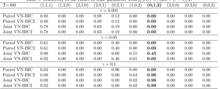
4.3 Sensitivity to the choice of scale parameter

In this section, we study the sensitivity of the performance of our procedures to the choice of scale parameters in the logistic transition function. We generate the arti…cial data using

y1t = y1t 1+"1t;

y2t = c0+ 0t;

y3t = (c0+ 0t)G( ; T) + (c1+ 1t)(1 G( ; T))

whereG( ; T)is a logistic transition function de…ned in section 2 and"1t=iidN(0;1),c= 0:5, 0 = 2,

= 0:5;and ₁ = 0:5. This model gives(r1; r2) = (0;1). As is noted in the previous sections, the scale

parameter controls the speed of transition. As approaches in…nity, the logistic function collapses to a index function I(t > T): On the other hand, as goes to zero, the smooth transition trend model

approaches to a linear trend. In this scenario, we can always …nd the linear combination that eliminates the trend function. Therefore, we expect that, when becomes smaller, it would be di¢ cult for our

3_{We also run simuation for other cases with AIC type and HQ type penalties. When sample size is large, however, they} are outperformed by the procedures with BIC type penalties.

(19)

procedure to identify the nonlinear deterministic trend from the linear trend.

Table 6 and Table 7 present the simulation results with fHP(r) = 2r(2m+r 1) and fCP(r) =

r(2m+ (r+ 1)=2)given di¤erent choices of the scale parameter _{2 f}0:001;0:05;0:1_g: The results are consistent with our prediction in direction.

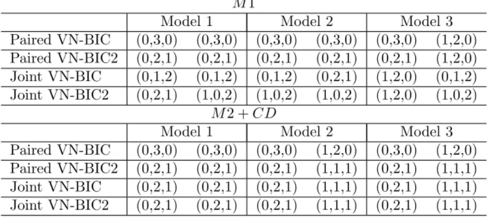
5 Application

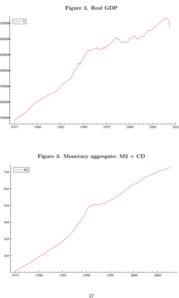
The simulation results in the previous section show that our procedures perform well in various ex-perimental set-ups. In this section, we apply our procedures to the Japanese money demand function to investigate the cotrending relations among money demand, income and interest rate. A seasonally adjusted quarterly series of real GDP, two de…nitions of monetary aggregates, M1 and M2 +CD, the

call rate are plotted in Figures 2 to 5. The …gures show the possibility of kinked deterministic trends in these variables.

We follow Bae, Kakkar and Ogaki (2006) and consider following three di¤erent speci…cations of money demand functions,

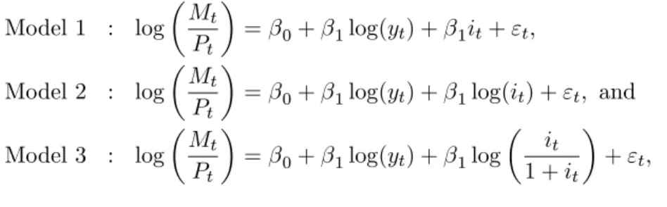
Model 1 : log Mt

Pt

= ₀+ ₁log(yt) + 1it+"t;

Model 2 : log Mt

Pt

= ₀+ ₁log(yt) + 1log(it) +"t; and

Model 3 : log Mt

Pt

= ₀+ ₁log(yt) + 1log

it

1 +it

+"t;

where Mt is the money demand, Pt is the aggregate price level, yt is real GDP and it is the nominal

interest rate.

We apply both paired and joint cotrending rank selection procedures to the vectors(log(Mt=Pt);log(yt); it),

(log(Mt=Pt);log(yt);log(it)), and (log(Mt=Pt);log(yt);log(it=(1 +it)) using the sample spanning from

(20)

is used. Table 8 reports the empirical results for all three di¤erent speci…cations of the functional form for interest elasticity of money demand. The results are somewhat mixed depending on the choice of the penalty of the criteria and the model of money demand.

Overall, however, we have more cases of choosing cotrending with r1 = 1 when Models 2 and 3

are used along with the penalty function fCP(r) =r(2m+ (r+ 1)=2). Bae, Kakkar and Ogaki (2006)

argue that the nonlinear functional forms (Models 2 and 3) are more appropriate for the Japanese long-run money demand. In that case, we have a stronger result in supporting the presence of cotrending relationship among these variables.

6 Conclusion

This paper has proposed a model-free cotrending rank selection procedure when both stochastic and nonlinear deterministic trends are present in a multivariate system. The procedure selects two types of cotrending rank by minimizing a new criterion based on the generalized von Neumann ratio. Our approach is invariant to linear transformation of data, robust to misspeci…cation of the model, and consistent under very general conditions. Monte Carlo experiments have suggested good …nite sample performance of the proposed procedure. Empirical applications to the money demand function in Japan have also suggested the usefulness of our procedure in detecting the cotrending relationships when there exists nonlinear deterministic trends in data.

(21)

Appendix

Proof of Lemma 1:

We want to show that b1, ,br1 is Op(1) but is not op(1), br1+1, ,br2 is Op(T

1₎ _{but is not}

op(T 1), and br2+1, ,bm is Op(T

2₎ _{but is not} _o

p(T 2)if all the eigenvalues of S111S00 are arranged

in a descending order. We employ the data matrix notation, Y0 = [y1; ; yT],D0 = [d1; ; dT] and

S0 = [s1; ; sT].

We have constructed an orthogonal full rank matrix[B_? B2 B1]in Assumption 1 and further de…ne

M11=B

0

S11B; and M00=B

0 S00B

Due to the orthogonality of the matrix [B_? B2 B1], the eigenvalues of S111S00 arise as the same

solutions to

det( M11 M00) = 0:

Our proof can be established in the following two steps. Step 1:

We assume G= limT!1T 3PtT=1dtd0t exists andT 3

PT

t=1dtd0t Gis O(T 1=2). The eigenvalues

of T2_M 1

11 M00 are equivalent to the eigenvalues

0

sthat solve

det( T 2M11 M00) = 0

For the matrixT 2_M

11, the only block matrix that is not equal to zero isB

0 ?Y

0

Y B_?, which converge toB_?0 GB_? under Assumption 1. Because the eigenvalues are continuous functions of the matrix,

p lim

T !1 i(T

2_M 1

11 M00) = i(p lim

T !1T

2_M 1 11 M00):

(22)

It can be easily shown thatM00isOp(1)but is notop(1). Therefore, for i=r2+ 1; ; m;we are led to

i(T2M111M00) =Op(1)but is not op(1):

This leads to the result that T2bi isOp(1)but notop(1)fori=r2+ 1; ; m:

Step 2:

Let DT =diag[Im r2; T

1=2_I

r2];the roots of

det( T 2M11 M00) = 0

are equivalent to

det(DT T 2M11 M00 DT) = 0 (2)

The matrix T 2M11 can be rewritten as

0 @

T 3B_?0 Y0Y B_? T 3B_?0 Y0Y[ B2 B1 ]

T 3[ B

0

2

B₁0 ]Y 0

Y B_? T 3[ B

0

2

B₁0 ]Y 0

Y[ B2 B1 ]

1 A;

and we denote

Ya= T 3B

0 ?Y

0

Y B_? B_?0 Y0 Y B_?0 ;

Yb= T 2

B0₂Y0Y B2 B02Y

0 Y B1

B0₁Y0Y B2 B01Y

0 Y B1

T B0₂ Y0 Y B2 T1=2B20 Y

0 Y B1

T1=2B₁0 Y0 Y B2 T B10 Y

0 Y B1

;

and

Yc = T

5 2 B

0

2Y

0 Y B_? B0₁Y0Y B_? T

1=2 B

0

2 Y

0

Y B_? B0₁ Y0 Y B_? :

(23)

Then equation (2) is rewritten as

det(Ya) det[Yb Y

0

cYa 1Yc] = 0 (3)

The …rst determinant can on the LHS of (3) cannot be equal to zero, implying the second determinant must be zero. Concerning the …rst part of Yb;only its …rst r2 r2 diagonal block is nonzero, and the

second part of Yb and Y

0

cYa 1Yc is Op(T) but is not op(T):Hence, we are led to

det( iT 2B

0

1Y

0

Y B1 Op(T)) = 0

for i = r1+ 1; ; r2. While we let T goes to in…nity and the solutions i solves the above equation

satis…es

i(T2M111M00) =Op(T) but is notop(T) fori=r1+ 1; ; r2:

Therefore, one can conclude that bi is Op(T 1) but is not op(T 1) fori=r1+ 1; ; r2. Analogously,

one can show thatbi isOp(1)but is not op(1)fori= 1; ; r1.

Proof of Proposition 2.

(i) Letr1be the true cotrending rank, which is estimated by minimization ofV N1(r1)for0 r1 m:

To check the consistency of this estimator, we need to showV N(r₁0)> V N(r1)if r

0

1 is not equal to the

true cotrending rankr1:

When r0₁< r1,

V N1(r

0

1) V N1(r1) =

r1 X

i=r0₁+1

(24)

In order to consistently selectr1 with probability 1 as T ! 1;we need

r1 X

i=r0₁+1

b_i+ (f(r0₁) f(r1))CTT 1>0; asT ! 1:

From Proposition 1, we know the …rst term is a positive number that is bounded away from zero and the second term is a negative number of order O(CTT 1): As long asCTT 1 ! 0 asT ! 1;the

above inequality holds and we are led to the conclusion thatV N1(r

0

1)> V N1(r1) when r

0

1 < r1:

When r0₁> r1,

V N1(r

0

1) V N1(r1) =

r0₁

X

i=r1+1

b_i+ (f(r₁0) f(r1))CTT 1

From Proposition 1, we know thatbi isOp(T 1)but is notop(T 1)fori=r1+ 1; r2;By multiplying

both sides by T; we have

T V N1(r

0

1) V N1(r1) = T

r0₁

X

i=r1+1

b_i+ (f(r0₁) f(r1))CT:

As long as CT ! 1 as T ! 1, the second term on the right hand side dominates, which leads to

V N1(r10)> V N1(r1)whenr01> r1. Thus the consistency ofV N1(r1) in selecting true cotrending rank is

established. Analogously, one can establish the consistency of the estimator of the true weak cotrending rank byV N2(r2):

(ii) To show the consistency of the joint selection procedure, consider all the possible cases as follows. Case 1: r0₁ < r1;

We have

V N(r0₁; r0₂) V N(r1; r2) =

p

T

r1 X

i=r0₁+1

b_i+Op(

CT

T );

where bi fori=r

0

1+ 1; ; r1 isOp(1)but is not op(1):

(25)

when r₁0 < r1:

Case 2: r0₁ > r1:

V N(r0₁; r₂0) V N(r1; r2) =

p

T

r0₁

X

i=r1+1

b_i+ (f(r₁0) f(r1))

CT

T +Op( CT

T2);

where bi is Op(T 1)fori=r1+ 1; ; m:

The dominant term in the above equation is(f(r0₁) f(r1))C_TT provided thatpCT_T ! 1, the inequality

V N(r0₁; r0₂)> V N(r1; r2)holds in this case.

Case 3: r0₁ =r1:

When r0₂> r2;

V N(r₁0; r₂0) V N(r1; r2) =

p

T

r₂0

X

i=r2+1

b_i+ (f(r0₂) f(r1))

C_T0 T2;

where bi is Op(T 2)forr

0

2+ 1; ; m:

Then, we have

T2 V N(r₁0; r₂0) V N(r1; r2) =

p

T

r₂0

X

i=r2+1

T2bi+ (f(r

0

2) f(r2))C

0

T:

Provided that _pCT

T ! 1, the dominant term is (f(r

0

2) f(r2))C

0

T, which is greater than zero. Hence

V N(r0₁; r0₂)> V N(r1; r2)in this case.

When r0₂< r2;

V N(r0₁; r₂0) V N(r1; r2) =

p

T

r2 X

i=r0₂+1

b_i+ (f(r0₂) f(r2))

C_T0 T2:

(26)

provided that C

0 T

T !0:HenceV N(r

0

1; r

0

2)> V N(r1; r2) in this case.

Combining the conditions onCT andC

0

T , for all the preceding cases, it follows that the joint selection

(27)

References

[1] Bacon, D. W., Watts, D. G., 1971. Estimating the transition between two intersecting straight lines.

Biometrika 58, 525–534.

[2] Bae, Y., Kakkar, V., Ogaki, M., 2006. Money demand in Japan and nonlinear cointegration.Journal of Money, Credit, and Banking 38, 1659-1667.

[3] Bai, J., Ng, S., 2002. Determine the number of factors in approximate factor models.Econometrica

70, 191-221.

[4] Bai, J., Ng, S., 2004. A PANIC attack on unit roots and cointegration.Econometrica 72, 1127-1177.

[5] Bierens, H. J., 2000. Nonparametric nonlinear co-trending analysis, with an application to in‡ation and interest in the U.S..Journal of Business and Economic Statistics 18, 323–337.

[6] Cheng, X., Phillips, P. C. B., 2009. Semiparametric cointegrating rank selection. Econometrics Journal 12, S83–S104.

[7] Clements, M. P., Hendry, D. F., 1999. On winning forecasting competitions in economics. Spanish Economic Review 1, 123–160.

[8] Engle, R. F., Granger, C. W. J., 1987. Cointegration and error correction: Representation, estima-tion, and testing.Econometrica 55, 251-276.

[9] Engle, R. F., Kozicki, S., 1993. Testing for common features. Journal of Business & Economic Statistics 11, 369-380.

[10] Granger, C. W. J., Teräsvirta, T., 1993. Modelling nonlinear economic relationships. Oxford Uni-versity Press.

(28)

[11] Greenaway, D., Leybourne, S., Sapsford, D., 1997. Modeling growth (and liberalization) using smooth transitions analysis.Economic Inquiry 35, 798-814

[12] Harris, D., Poskitt, D. S., 2004. Determination of cointegrating rank in partially non-stationary process via a generalised von-Neumann criterion.Econometrics Journal 7, 191-217.

[13] Hatanaka, M., 2000. How to determine the number of relations among deterministic trends., The Japanese Economic Review 51, 349-373.

[14] Hatanaka, M., Yamada, H., 2003. Co-trending: A Statistical System Analysis of Economic Trends, Springer.

[15] Hendry, D. F., Mizon, G. E., 1998. Exogeneity, causality, and co-breaking in economic policy analysis of a small econometric model of money in the UK.Empirical Economics 23, 267-294.

[16] Johansen, S., 1991. Estimation and hypothesis test of cointegration vectors in Gaussian vector autoregressive models.Econometrica 59, 1551-1580.

[17] Mills, T., 2003. Modelling Trends and Cycles in Economics Time Series, Palgrave Macmillan.

[18] Nelson, C. R., Plosser C. R., 1982. Trends and random walks in macroeconomic time series: some evidence and implications.Journal of Monetary Economics 10, 139-162.

[19] Ogaki, M., Park, J. Y., 1998. A cointegration approach to estimating preference parameters.Journal of Econometrics 82, 107–134.

[20] Perron, P., 1989. The great crash, the oil price shock and the unit root hypothesis. Econometrica

57, 1361-1401.

[21] Perron, P., 1997. Further evidence from breaking trend functions in macroeconomic variables. Jour-nal of Econometrics 80, 355-385.

(29)

[22] Rappoport, P., Reichlin, L., 1989. Segmented trends and non-stationary time series. Economic Journal 99, 168-77.

[23] Shintani, M., 2001. A simple cointegrating rank test without vector autoregression. Journal of Econometrics 105, 337-362.

[24] Stock, J. H., Watson, M. W., 1988. Testing for common trends.Journal of the American Statistical Association 83, 1097-1107.

[25] Teräsvirta, T., 1994. Speci…cation, estimation, and evaluation of smooth transition autoregressive models.Journal of the American Statistical Association 89, 208-218.

(30)

Table 1. Two dimensional cointegrating rank selection

T = 100 T = 400

DGP:r1= 0 DGP: r1= 0

r1= 0 r1= 1 r1= 2 r1= 0 r1= 1 r1= 2

RRR-AIC 0.49 0.39 0.12 RRR-AIC 0.52 0.37 0.11

RRR-BIC 0.88 0.11 0.01 RRR-BIC 0.95 0.05 0.00

RRR-HQ 0.35 0.47 0.19 RRR-HQ 0.46 0.41 0.13

VN-AIC 0.98 0.02 0.00 VN-AIC 0.97 0.03 0.00

VN-BIC 1.00 0.00 0.00 VN-BIC 1.00 0.00 0.00

VN-HQ 0.93 0.07 0.00 VN-HQ 0.95 0.05 0.00

r1= 0 r1= 1 r1= 2 r1= 0 r1= 1 r1= 2

RRR-AIC 0.00 0.78 0.22 RRR-AIC 0.00 0.76 0.24

RRR-BIC 0.00 0.94 0.06 RRR-BIC 0.00 0.96 0.04

RRR-HQ 0.00 0.71 0.29 RRR-HQ 0.00 0.73 0.27

VN-AIC 0.00 1.00 0.00 VN-AIC 0.00 1.00 0.00

VN-BIC 0.05 0.95 0.00 VN-BIC 0.00 1.00 0.00

VN-HQ 0.00 1.00 0.00 VN-HQ 0.00 1.00 0.10

r1= 0 r1= 1 r1= 2 r1= 0 r1= 1 r1= 2

RRR-AIC 0.00 0.25 0.75 RRR-AIC 0.00 0.00 1.00

RRR-BIC 0.05 0.73 0.22 RRR-BIC 0.00 0.02 0.98

RRR-HQ 0.00 0.14 0.86 RRR-HQ 0.00 0.00 1.00

VN-AIC 0.00 0.39 0.61 VN-AIC 0.00 0.00 1.00

VN-BIC 0.00 0.95 0.05 VN-BIC 0.00 0.06 0.94

VN-HQ 0.00 0.19 0.81 VN-HQ 0.00 0.00 1.00

(31)

Table 2. Simulation results on cotrending rank selection withfHP(r) = 2r(2m r+ 1)

T=100 (1,1,1) (1,2,0) (2,1,0) (2,0,1) (0,2,1) (1,0,2) (0,1,2) (3,0,0) (0,3,0) (0,0,3)

Paired VN-BIC 0.97 0.00 0.00 0.03 0.00 0.00 0.00 0.00 0.00 0.00

Paired VN-BIC2 0.97 0.00 0.00 0.03 0.00 0.00 0.00 0.00 0.00 0.00

Joint VN-BIC 0.94 0.00 0.00 0.02 0.00 0.04 0.00 0.00 0.00 0.00

Joint VN-BIC2 0.98 0.00 0.00 0.02 0.00 0.00 0.00 0.00 0.00 0.00

T=100 (1,1,1) (1,2,0) (2,1,0) (2,0,1) (0,2,1) (1,0,2) (0,1,2) (3,0,0) (0,3,0) (0,0,3)

Paired VN-BIC 0.00 0.93 0.07 0.00 0.00 0.00 0.00 0.00 0.00 0.00

Paired VN-BIC2 0.93 0.00 0.00 0.07 0.00 0.00 0.00 0.00 0.00 0.00

Joint VN-BIC 0.46 0.49 0.02 0.03 0.00 0.01 0.00 0.00 0.00 0.00

Joint VN-BIC2 0.04 0.92 0.04 0.01 0.00 0.00 0.00 0.00 0.00 0.00

T=100 (1,1,1) (1,2,0) (2,1,0) (2,0,1) (0,2,1) (1,0,2) (0,1,2) (3,0,0) (0,3,0) (0,0,3)

Paired VN-BIC 0.00 0.00 0.93 0.00 0.00 0.00 0.00 0.07 0.00 0.00

Paired VN-BIC2 0.00 0.00 0.00 0.93 0.00 0.00 0.00 0.00 0.00 0.07

Joint VN-BIC 0.00 0.00 0.53 0.42 0.00 0.00 0.00 0.05 0.00 0.00

Joint VN-BIC2 0.00 0.00 0.89 0.06 0.00 0.00 0.00 0.05 0.00 0.00

T=100 (1,1,1) (1,2,0) (2,1,0) (2,0,1) (0,2,1) (1,0,2) (0,1,2) (3,0,0) (0,3,0) (0,0,3)

Paried VN-BIC 0.00 0.00 0.00 1.00 0.00 0.00 0.00 0.00 0.00 0.00

Paired VN-BIC2 0.00 0.00 0.00 1.00 0.00 0.00 0.00 0.00 0.00 0.00

Joint VN-BIC 0.00 0.00 0.00 1.00 0.00 0.00 0.00 0.00 0.00 0.00

Joint VN-BIC2 0.00 0.00 0.00 1.00 0.00 0.00 0.00 0.00 0.00 0.00

T=100 (1,1,1) (1,2,0) (2,1,0) (2,0,1) (0,2,1) (1,0,2) (0,1,2) (3,0,0) (0,3,0) (0,0,3)

Paried VN-BIC 0.07 0.00 0.00 0.00 0.93 0.00 0.00 0.00 0.00 0.00

Paired VN-BIC2 0.07 0.00 0.00 0.00 0.93 0.00 0.00 0.00 0.00 0.00

Joint VN-BIC 0.04 0.00 0.00 0.00 0.94 0.00 0.01 0.00 0.00 0.00

Joint VN-BIC2 0.04 0.00 0.00 0.00 0.96 0.00 0.00 0.00 0.00 0.00

T=100 (1,1,1) (1,2,0) (2,1,0) (2,0,1) (0,2,1) (1,0,2) (0,1,2) (3,0,0) (0,3,0) (0,0,3)

Paried VN-BIC 1.00 0.00 0.00 0.00 0.00 0.00 0.00 0.00 0.00 0.00

Paired VN-BIC2 0.00 0.00 0.00 0.00 0.00 1.00 0.00 0.00 0.00 0.00

Joint VN-BIC 0.00 0.00 0.00 0.00 0.00 1.00 0.00 0.00 0.00 0.00

Joint VN-BIC2 0.00 0.00 0.00 0.00 0.00 1.00 0.00 0.00 0.00 0.00

T=100 (1,1,1) (1,2,0) (2,1,0) (2,0,1) (0,2,1) (1,0,2) (0,1,2) (3,0,0) (0,3,0) (0,0,3)

Paried VN-BIC 0.03 0.00 0.00 0.00 0.97 0.00 0.00 0.00 0.00 0.00

Paired VN-BIC2 0.00 0.00 0.00 0.00 0.00 0.03 0.97 0.00 0.00 0.00

Joint VN-BIC 0.00 0.00 0.00 0.00 0.00 0.02 0.98 0.00 0.00 0.00

Joint VN-BIC2 0.00 0.00 0.00 0.00 0.00 0.02 0.98 0.00 0.00 0.00

T=100 (1,1,1) (1,2,0) (2,1,0) (2,0,1) (0,2,1) (1,0,2) (0,1,2) (3,0,0) (0,3,0) (0,0,3)

Paried VN-BIC 0.00 0.00 0.00 0.00 0.00 0.00 0.00 1.00 0.00 0.00

Paired VN-BIC2 0.00 0.00 0.00 0.00 0.00 0.00 0.00 0.00 0.00 1.00

Joint VN-BIC 0.00 0.00 0.00 0.00 0.00 0.00 0.00 1.00 0.00 0.00

Joint VN-BIC2 0.00 0.00 0.00 0.00 0.00 0.00 0.00 1.00 0.00 0.00

T=100 (1,1,1) (1,2,0) (2,1,0) (2,0,1) (0,2,1) (1,0,2) (0,1,2) (3,0,0) (0,3,0) (0,0,3)

Paried VN-BIC 0.00 0.09 0.01 0.00 0.00 0.00 0.00 0.00 0.91 0.00

Paired VN-BIC2 0.09 0.00 0.00 0.00 0.91 0.00 0.00 0.00 0.00 0.00

Joint VN-BIC 0.03 0.02 0.00 0.00 0.20 0.00 0.00 0.00 0.74 0.00

Joint VN-BIC2 0.00 0.05 0.00 0.00 0.00 0.00 0.00 0.00 0.94 0.00

T=100 (1,1,1) (1,2,0) (2,1,0) (2,0,1) (0,2,1) (1,0,2) (0,1,2) (3,0,0) (0,3,0) (0,0,3)

Paried VN-BIC 0.00 0.00 0.00 0.00 1.00 0.00 0.00 0.00 0.00 0.00

Paired VN-BIC2 0.00 0.00 0.00 0.00 0.00 0.00 0.00 0.00 0.00 1.00

Joint VN-BIC 0.00 0.00 0.00 0.00 0.00 0.00 0.00 0.00 0.00 1.00

(32)

Table 3. Simulation results on cotrending rank selection withfHP(r) = 2r(2m r+ 1)

T=400 (1,1,1) (1,2,0) (2,1,0) (2,0,1) (0,2,1) (1,0,2) (0,1,2) (3,0,0) (0,3,0) (0,0,3)

Paired VN-BIC 0.99 0.00 0.00 0.01 0.00 0.00 0.00 0.00 0.00 0.00

Paired VN-BIC2 0.99 0.00 0.00 0.01 0.00 0.00 0.00 0.00 0.00 0.00

Joint VN-BIC 0.98 0.00 0.00 0.01 0.00 0.00 0.00 0.00 0.00 0.00

Joint VN-BIC2 0.99 0.00 0.00 0.01 0.00 0.00 0.00 0.00 0.00 0.00

T=400 (1,1,1) (1,2,0) (2,1,0) (2,0,1) (0,2,1) (1,0,2) (0,1,2) (3,0,0) (0,3,0) (0,0,3)

Paired VN-BIC 0.00 0.98 0.02 0.00 0.00 0.00 0.00 0.00 000 0.00

Paired VN-BIC2 0.98 0.00 0.00 0.02 0.00 0.00 0.00 0.00 0.00 0.00

Joint VN-BIC 0.23 0.75 0.01 0.01 0.00 0.00 0.00 0.00 0.00 0.00

Joint VN-BIC2 0.00 0.98 0.02 0.00 0.00 0.00 0.00 0.00 0.00 0.00

T=400 (1,1,1) (1,2,0) (2,1,0) (2,0,1) (0,2,1) (1,0,2) (0,1,2) (3,0,0) (0,3,0) (0,0,3)

Paired VN-BIC 0.00 0.00 0.97 0.00 0.00 0.00 0.00 0.03 0.00 0.00

Paired VN-BIC2 0.00 0.00 0.00 0.97 0.00 0.00 0.00 0.00 0.00 0.03

Joint VN-BIC 0.00 0.00 0.70 0.27 0.00 0.00 0.00 0.03 0.00 0.00

Joint VN-BIC2 0.00 0.00 0.96 0.02 0.00 0.00 0.00 0.03 0.00 0.00

T=400 (1,1,1) (1,2,0) (2,1,0) (2,0,1) (0,2,1) (1,0,2) (0,1,2) (3,0,0) (0,3,0) (0,0,3)

Paried VN-BIC 0.00 0.00 0.00 1.00 0.00 0.00 0.00 0.00 0.00 0.00

Paired VN-BIC2 0.00 0.00 0.00 1.00 0.00 0.00 0.00 0.00 0.00 0.00

Joint VN-BIC 0.00 0.00 0.00 1.00 0.00 0.00 0.00 0.00 0.00 0.00

Joint VN-BIC2 0.00 0.00 0.00 1.00 0.00 0.00 0.00 0.00 0.00 0.00

T=400 (1,1,1) (1,2,0) (2,1,0) (2,0,1) (0,2,1) (1,0,2) (0,1,2) (3,0,0) (0,3,0) (0,0,3)

Paried VN-BIC 0.02 0.00 0.00 0.00 0.98 0.00 0.00 0.00 0.00 0.00

Paired VN-BIC2 0.02 0.00 0.00 0.00 0.98 0.00 0.00 0.00 0.00 0.00

Joint VN-BIC 0.01 0.00 0.00 0.00 0.99 0.00 0.00 0.00 0.00 0.00

Joint VN-BIC2 0.01 0.00 0.00 0.00 0.99 0.00 0.00 0.00 0.00 0.00

T=400 (1,1,1) (1,2,0) (2,1,0) (2,0,1) (0,2,1) (1,0,2) (0,1,2) (3,0,0) (0,3,0) (0,0,3)

Paried VN-BIC 1.00 0.00 0.00 0.00 0.00 0.00 0.00 0.00 0.00 0.00

Paired VN-BIC2 0.00 0.00 0.00 0.00 0.00 1.00 0.00 0.00 0.00 0.00

Joint VN-BIC 0.00 0.00 0.00 0.00 0.00 1.00 0.00 0.00 0.00 0.00

Joint VN-BIC2 0.00 0.00 0.00 0.00 0.00 1.00 0.00 0.00 0.00 0.00

T=400 (1,1,1) (1,2,0) (2,1,0) (2,0,1) (0,2,1) (1,0,2) (0,1,2) (3,0,0) (0,3,0) (0,0,3)

Paried VN-BIC 0.01 0.00 0.00 0.00 0.99 0.00 0.00 0.00 0.00 0.00

Paired VN-BIC2 0.00 0.00 0.00 0.00 0.00 0.01 0.99 0.00 0.00 0.00

Joint VN-BIC 0.00 0.00 0.00 0.00 0.00 0.01 0.99 0.00 0.00 0.00

Joint VN-BIC2 0.00 0.00 0.00 0.00 0.00 0.01 0.99 0.00 0.00 0.00

T=400 (1,1,1) (1,2,0) (2,1,0) (2,0,1) (0,2,1) (1,0,2) (0,1,2) (3,0,0) (0,3,0) (0,0,3)

Paried VN-BIC 0.00 0.00 0.00 0.00 0.00 0.00 0.00 1.00 0.00 0.00

Paired VN-BIC2 0.00 0.00 0.00 0.00 0.00 0.00 0.00 1.00 0.00 0.00

Joint VN-BIC 0.00 0.00 0.00 0.00 0.00 0.00 0.00 1.00 0.00 0.00

Joint VN-BIC2 0.00 0.00 0.00 0.00 0.00 0.00 0.00 1.00 0.00 0.00

T=400 (1,1,1) (1,2,0) (2,1,0) (2,0,1) (0,2,1) (1,0,2) (0,1,2) (3,0,0) (0,3,0) (0,0,3)

Paried VN-BIC 0.00 0.02 0.00 0.00 0.00 0.00 0.00 0.00 0.98 0.00

Paired VN-BIC2 0.02 0.00 0.00 0.00 0.98 0.00 0.00 0.00 0.00 0.00

Joint VN-BIC 0.00 0.01 0.00 0.00 0.07 0.00 0.00 0.00 0.92 0.00

Joint VN-BIC2 0.00 0.01 0.00 0.00 0.00 0.00 0.00 0.00 0.99 0.00

T=400 (1,1,1) (1,2,0) (2,1,0) (2,0,1) (0,2,1) (1,0,2) (0,1,2) (3,0,0) (0,3,0) (0,0,3)

Paried VN-BIC 0.00 0.00 0.00 0.00 0.00 0.00 1.00 0.00 0.00 0.00

Paired VN-BIC2 0.00 0.00 0.00 0.00 0.00 0.00 0.00 0.00 0.00 1.00

Joint VN-BIC 0.00 0.00 0.00 0.00 0.00 0.00 0.00 0.00 0.00 1.00

(33)

Table 4. Simulation results on cotrending rank selection withfCP(r) =r(2m+ (r+ 1)=2)

T=100 (1,1,1) (1,2,0) (2,1,0) (2,0,1) (0,2,1) (1,0,2) (0,1,2) (3,0,0) (0,3,0) (0,0,3)

Paired VN-BIC 0.66 0.00 0.00 0.35 0.00 0.00 0.00 0.00 0.00 0.00

Paired VN-BIC2 0.66 0.00 0.00 0.35 0.00 0.00 0.00 0.00 0.00 0.00

Joint VN-BIC 0.72 0.00 0.00 0.28 0.00 0.00 0.00 0.00 0.00 0.00

Joint VN-BIC2 0.72 0.00 0.00 0.28 0.00 0.00 0.00 0.00 0.00 0.00

T=100 (1,1,1) (1,2,0) (2,1,0) (2,0,1) (0,2,1) (1,0,2) (0,1,2) (3,0,0) (0,3,0) (0,0,3)

Paired VN-BIC 0.00 0.50 0.48 0.00 0.00 0.00 0.00 0.02 000 0.00

Paired VN-BIC2 0.00 0.50 0.48 0.00 0.00 0.00 0.00 0.02 0.00 0.00

Joint VN-BIC 0.08 0.50 0.32 0.09 0.00 0.00 0.00 0.01 0.00 0.00

Joint VN-BIC2 0.00 0.58 0.40 0.00 0.00 0.00 0.00 0.01 0.00 0.00

T=100 (1,1,1) (1,2,0) (2,1,0) (2,0,1) (0,2,1) (1,0,2) (0,1,2) (3,0,0) (0,3,0) (0,0,3)

Paired VN-BIC 0.00 0.00 0.85 0.00 0.00 0.00 0.00 0.15 0.00 0.00

Paired VN-BIC2 0.00 0.00 0.85 0.00 0.00 0.00 0.00 0.15 0.00 0.03

Joint VN-BIC 0.00 0.00 0.76 0.12 0.00 0.00 0.00 0.12 0.00 0.00

Joint VN-BIC2 0.00 0.00 0.89 0.00 0.00 0.00 0.00 0.11 0.00 0.00

T=100 (1,1,1) (1,2,0) (2,1,0) (2,0,1) (0,2,1) (1,0,2) (0,1,2) (3,0,0) (0,3,0) (0,0,3)

Paried VN-BIC 0.00 0.00 0.00 1.00 0.00 0.00 0.00 0.00 0.00 0.00

Paired VN-BIC2 0.00 0.00 0.00 1.00 0.00 0.00 0.00 0.00 0.00 0.00

Joint VN-BIC 0.00 0.00 0.00 1.00 0.00 0.00 0.00 0.00 0.00 0.00

Joint VN-BIC2 0.00 0.00 0.00 1.00 0.00 0.00 0.00 0.00 0.00 0.00

T=100 (1,1,1) (1,2,0) (2,1,0) (2,0,1) (0,2,1) (1,0,2) (0,1,2) (3,0,0) (0,3,0) (0,0,3)

Paried VN-BIC 0.63 0.00 0.00 0.16 0.20 0.00 0.00 0.00 0.00 0.00

Paired VN-BIC2 0.63 0.00 0.00 0.16 0.20 0.00 0.00 0.00 0.00 0.00

Joint VN-BIC 0.60 0.00 0.00 0.12 0.28 0.00 0.00 0.00 0.00 0.00

Joint VN-BIC2 0.60 0.00 0.00 0.11 0.29 0.00 0.00 0.00 0.00 0.00

T=100 (1,1,1) (1,2,0) (2,1,0) (2,0,1) (0,2,1) (1,0,2) (0,1,2) (3,0,0) (0,3,0) (0,0,3)

Paried VN-BIC 1.00 0.00 0.00 0.00 0.00 0.00 0.00 0.00 0.00 0.00

Paired VN-BIC2 0.00 0.00 0.00 0.00 0.00 1.00 0.00 0.00 0.00 0.00

Joint VN-BIC 0.00 0.00 0.00 0.00 0.00 1.00 0.00 0.00 0.00 0.00

Joint VN-BIC2 0.00 0.00 0.00 0.00 0.00 1.00 0.00 0.00 0.00 0.00

T=100 (1,1,1) (1,2,0) (2,1,0) (2,0,1) (0,2,1) (1,0,2) (0,1,2) (3,0,0) (0,3,0) (0,0,3)

Paried VN-BIC 0.55 0.00 0.00 0.00 0.45 0.00 0.00 0.00 0.00 0.00

Paired VN-BIC2 0.33 0.00 0.00 0.00 0.15 0.22 0.30 0.00 0.00 0.00

Joint VN-BIC 0.00 0.00 0.00 0.00 0.00 0.47 0.53 0.00 0.00 0.00

Joint VN-BIC2 0.47 0.00 0.00 0.00 0.54 0.00 0.00 0.00 0.00 0.00

T=100 (1,1,1) (1,2,0) (2,1,0) (2,0,1) (0,2,1) (1,0,2) (0,1,2) (3,0,0) (0,3,0) (0,0,3)

Paried VN-BIC 0.00 0.00 0.00 0.00 0.00 0.00 0.00 1.00 0.00 0.00

Paired VN-BIC2 0.00 0.00 0.00 0.00 0.00 0.00 0.00 1.00 0.00 1.00

Joint VN-BIC 0.00 0.00 0.00 0.00 0.00 0.00 0.00 1.00 0.00 0.00

Joint VN-BIC2 0.00 0.00 0.00 0.00 0.00 0.00 0.00 1.00 0.00 0.00

T=100 (1,1,1) (1,2,0) (2,1,0) (2,0,1) (0,2,1) (1,0,2) (0,1,2) (3,0,0) (0,3,0) (0,0,3)

Paried VN-BIC 0.00 0.60 0.24 0.00 0.00 0.00 0.00 0.00 0.16 0.00

Paired VN-BIC2 0.00 0.60 0.24 0.00 0.98 0.00 0.00 0.00 0.16 0.00

Joint VN-BIC 0.13 0.48 0.12 0.05 0.02 0.00 0.00 0.00 0.20 0.00

Joint VN-BIC2 0.00 0.61 0.17 0.00 0.00 0.00 0.00 0.00 0.23 0.00

T=100 (1,1,1) (1,2,0) (2,1,0) (2,0,1) (0,2,1) (1,0,2) (0,1,2) (3,0,0) (0,3,0) (0,0,3)

Paried VN-BIC 0.00 0.00 0.00 0.00 1.00 0.00 0.00 0.00 0.00 0.00

Paired VN-BIC2 0.00 0.00 0.00 0.00 0.00 0.00 1.00 0.00 0.00 0.00

Joint VN-BIC 0.00 0.00 0.00 0.00 0.00 0.00 1.00 0.00 0.00 0.00

(34)

Table 5. Simulation results on cotrending rank selection withfCP(r) =r(2m+ (r+ 1)=2)

T=400 (1,1,1) (1,2,0) (2,1,0) (2,0,1) (0,2,1) (1,0,2) (0,1,2) (3,0,0) (0,3,0) (0,0,3)

Paired VN-BIC 0.82 0.00 0.00 0.18 0.00 0.00 0.00 0.00 0.00 0.00

Paired VN-BIC2 0.82 0.00 0.00 0.18 0.00 0.00 0.00 0.00 0.00 0.00

Joint VN-BIC 0.84 0.00 0.00 0.17 0.00 0.00 0.00 0.00 0.00 0.00

Joint VN-BIC2 0.84 0.00 0.00 0.16 0.00 0.00 0.00 0.00 0.00 0.00

T=400 (1,1,1) (1,2,0) (2,1,0) (2,0,1) (0,2,1) (1,0,2) (0,1,2) (3,0,0) (0,3,0) (0,0,3)

Paired VN-BIC 0.00 0.71 0.29 0.00 0.00 0.00 0.00 0.00 000 0.00

Paired VN-BIC2 0.00 0.71 0.29 0.00 0.00 0.00 0.00 0.00 0.00 0.00

Joint VN-BIC 0.04 0.69 0.24 0.02 0.00 0.00 0.00 0.00 0.00 0.00

Joint VN-BIC2 0.00 0.73 0.27 0.00 0.00 0.00 0.00 0.00 0.00 0.00

T=400 (1,1,1) (1,2,0) (2,1,0) (2,0,1) (0,2,1) (1,0,2) (0,1,2) (3,0,0) (0,3,0) (0,0,3)

Paired VN-BIC 0.00 0.00 0.91 0.00 0.00 0.00 0.00 0.09 0.00 0.00

Paired VN-BIC2 0.00 0.00 0.91 0.00 0.00 0.00 0.00 0.09 0.00 0.03

Joint VN-BIC 0.00 0.00 0.87 0.05 0.00 0.00 0.00 0.07 0.00 0.00

Joint VN-BIC2 0.00 0.00 0.93 0.00 0.00 0.00 0.00 0.07 0.00 0.00