Has US Shale Gas Reduced CO2 Emissions?

(1)

Has US Shale Gas Reduced CO

2

Emissions?

Examining recent changes in emissions from the US power sector and traded fossil fuels October 2012

Dr John Broderick & Prof Kevin Anderson Tyndall Manchester

University of Manchester Manchester M13 9PL

john.broderick@manchester.ac.uk

A research briefing commissioned by

This report is non-peer-reviewed and all views contained within are attributable to the authors and do not necessarily reflect those of researchers within the wider Tyndall Centre.

(2)

1

1 Executive Summary

Since 2007, the production of shale gas in large volumes has substantially reduced the wholesale price of natural gas in the US. This report examines the emissions savings in the US power sector, influenced by shale gas, and the concurrent trends in coal exports that may increase emissions in Europe and Asia.

Electricity generated by the combustion of natural gas is generally considered to have a lower emissions intensity per unit electricity than that generated by burning coal. The relative lifecycle carbon footprint of gas produced by hydraulic fracturing is contested and at present there is a shortage of independent primary data. However, trends in the absolute quantities of CO2 emissions from combustion are less problematic and no less important

when considering the implications of the US shale gas boom.

US CO2 emissions from domestic energy have declined by 8.6% since a peak in 2005, the

equivalent of 1.4% per year. Not all of this reduction has come in the power sector where shale gas has had most impact, and not all of the fuel switching has been due to the low price of gas. This report quantitatively explores the CO2 emissions consequences of fuel

switching in the US power sector using two simple methodologies. The analysis presented is conditional upon its internal assumptions, but provides an indication of the scale of

potential impacts.

It suggests that emissions avoided at a national scale due to fuel switching in the power sector may be up to half of the total reduction in US energy system CO2 emissions. The

suppression of gas prices through shale gas availability is a plausible causative mechanism for at least part of this reduction in emissions. However, the research presented here has not isolated the proportion of fuel switching due to price effects. Other studies note that between 35% and 50% of the difference between peak and present power sector emissions may be due to shale gas price effects. Renewable and nuclear electricity incentivised by other policies has also accounted for some of the changes in grid emissions. We estimate that their increase in output appears to have been about two thirds of the increase in gas generation.

There has been a substantial increase in coal exports from the US over this time period (2008-2011) and globally, coal consumption has continued to rise. As we discussed in our previous report (Broderick et al. 2011), without a meaningful cap on global carbon

emissions, the exploitation of shale gas reserves is likely to increase total emissions. For this not to be the case, consumption of displaced fuels must be reduced globally and remain suppressed indefinitely; in effect displaced coal must stay in the ground. The availability of shale gas does not guarantee this. Likewise, new renewable generating capacity may cause displacement without guaranteeing that coal is not burned, but it does not directly release carbon dioxide emissions through generation.

The calculations presented in this report suggest that more than half of the emissions avoided in the US power sector may have been exported as coal. In total, this export is equivalent to 340 MtCO2 emissions elsewhere in the world, i.e. 52% of the 650 MtCO2 of

(4)

3 A similar conclusion holds for ‘peak to present’ trends. The estimated additional 75 million short tons1 of coal exported from the US in 2011 will release 150 MtCO2 to the atmosphere

upon combustion. If added to the US CO2 output from fossil fuel combustion, the reduction

from peak emissions in 2005 would be 360 MtCO2, i.e. a 6.0% change over this whole period

or less than 1% per annum. This is far short of the rapid decarbonisation required to avoid dangerous climate change associated with a 2°C temperature rise.

1_{The US Energy Information Administration statistics record coal traded in short tons equivalent to 2000lbs,}

slightly lighter than both the metric tonne (2205lbs) and the long ton (2240lbs) used in the UK Imperial system. Units are taken directly from the original data source for ease of comparison and review.

(5)

4

2 Introduction

The production of ‘unconventional’ gas from shales, tight sandstones and coal beds promises to have a substantial impact on global energy systems in the coming decades. At present, the use of hydraulic fracturing as a production method is well developed only within the US fossil fuel industry. In the last few years, wholesale prices have fallen substantially as gas produced from shales and other unconventional reserves has become available in high volumes (Rogers 2011). The gas industry and its supporters claim that this growth in indigenous gas supply is positive from both energy security and climate change perspectives as it displaces imported gas or indigenous coal (Kuhn & Umbach 2011; Lovelock 2012).

Considering the wide abundance of unconventional gas resources and their presence in high demand economies, such as North America and China, there are many energy policy

makers, commentators and researchers who suggest that this supply will contribute to decarbonisation, with various qualifications (Helm 2011; The Economist 2012). However, having posed the question “Are We Entering a Golden Age of Gas?” in last year’s World Energy Outlook (2011) the IEA reported that this scenario would likely result in 3.5°C warming, well beyond what is generally regarded as dangerous climate change. This lead their Chief Economist, Dr Fatih Birol, to clarify that "We are not saying that it will be a golden age for humanity -- we are saying it will be a golden age for gas" (Harrabin 2012). In our previous research report (Broderick et al. 2011), we concluded that, in absence of wider policies, increasing production of any given fossil fuel was likely to result in an additional atmospheric burden and greater risk of dangerous climate change. Demand for energy of all kinds is growing and, as a scarce and essential resource, energy inevitably constrains the rate of economic growth. If new supply becomes available then there is a downward pressure on energy prices with a consequent rise in its consumption. In the case of shale gas, any putative benefit from the lower emissions intensity of natural gas over coal is therefore likely to be partially or fully negated through a rise in the consumption of fossil fuels as a whole. Climate change is an issue of absolute and not relative emissions, and any analysis that fails to respond to such an agenda risks seriously undermining action to mitigate emissions.

Building on such a system-level and scientifically-informed framing of climate change, this briefing considers the latest energy, trade and emissions statistics from the US and

addresses empirically the impact of shale gas on absolute emissions. The following questions structure the research presented in this report:

1. What has been the impact of shale gas on other fuels in the US?

a. Has it displaced coal in the power, domestic or industrial sectors? b. Has the price of coal altered?

c. Have imports and exports of coal changed? d. How has it interacted with other sources of gas? e. Have imports and exports of gas changed?

(6)

5 3. What has been the impact on CO2 emissions outside of the US? What are the

implications of global energy trends and international climate policies?

3 Is shale gas substituting for coal in the US energy system?

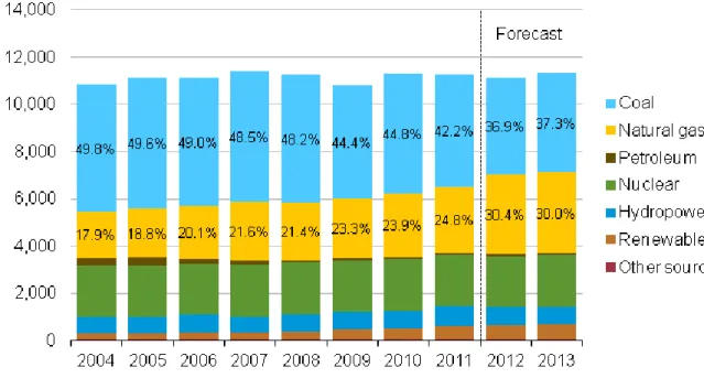
In April 2012 mild weather conditions reduced total demand for electricity in the US, with natural gas prices simultaneously falling to a ten year low. As a result, the proportion of electricity generation from gas was only fractionally below that of coal, an unprecedented situation.

Figure 1 US power generation by fuel source, EIA (2012)

Recent statistics presented by the US EIA show a number of trends in the relative consumption and prices of coal and gas. The following figures and analysis have been assembled from data within the Annual Energy Outlook 2012 (EIA 2012a), Quarterly Coal Report June 2012 (EIA 2012e), Short-Term Energy Outlook June 2012 (EIA 2012f) and the Electric Power Annual 2010 (EIA 2011). It is first worth reviewing the gas supply data, trends and credible expectations, and assessing the impact of shale gas production upon them.

(7)

6

Figure 2 Trend in US shale gas production volume

Total US natural gas production declined over the period 2001 to 2005, from 55bcf/day to 52bcf/day (1.6bcm/day to 1.5bcm/day), but subsequently grew strongly as shale gas wells came online in large numbers (Figure 2, above). Figure 3 illustrates this increase in absolute terms, pro-rating EIA shale production figures for processing losses and displaying the simultaneous reduction of non-shale gas production and net imports to the US. This

suggests that shale gas availability has not only substituted for coal in the US energy system but also other sources of gas. There is no physical or chemical reason to preferentially consume shale gas in one end use or another because of its chemical composition. It is not superior for home heating, power generation or petrochemical production; the major gaseous constituent, methane, can be fed directly into conventional natural gas distribution networks.

4

U.S. shale gas production has increased 14-fold in 10 years

0.0 0.5 1.0 1.5 2.0 2.5 3.0 3.5 4.0 4.5 5.0

2000 2001 2002 2003 2004 2005 2006 2007 2008 2009 2010

Antrim Barnett Fayetteville

Woodford Haynesville Marcellus Eagle Ford

Source: EIA, Lippman Consulting (2010 estimated)

annual shale gas production trillion cubic feet

(8)

7

Figure 3 US Gas production and imports

Indexing gas production to 2001 levels (Figure 4) illustrates the relative decline in imports as total gas consumption increases from 2006 onwards.

Figure 4 Indexed gas volumes

The most recent production statistics are not yet validated but 2011 gross shale gas production was reported at 66bcf/day (1.9bcm/day) and further increases are expected in coming years. The latest EIA Annual Energy Outlook (AEO) Reference Case (EIA 2012g) is based on shale gas increasing from 23% in 2010 to 49% of US production by 2035. In absolute terms, this would be over 25tcf (710bcm) total annual production, shifting the US from being a net gas importer to a net exporter of approximately 5% of its production by 2035.

0 0.2 0.4 0.6 0.8 1 1.2

R

e

la

ti

ve

v

al

ue

,

ind

e

xe

d

to

2

0

1

Indexed Gas Volumes

Dry gas production Net Imports Net Imports as % of consumption Consumption Non shale gas production

(9)

8 Over the last decade, US absolute natural gas consumption has grown nearly 10%, from 22 trillion cubic feet in 2001 to 24 trillion cubic feet in 2011. This rise is predominantly due to increased consumption in the power sector as described below in Section 3.1. The

wholesale gas price has not proceeded on a simple trajectory. Having peaked in 2005 and 2008 at around $9/MMBtu2, it fell back to less than half this price in 2009 and has continued as a low level since. At the time of writing, September 2012, the Henry Hub natural gas spot price is just below $3/MMBtu. This is partly due to the scale and productivity of US shale plays and partly the high value of oil fractions present in the output of some shale plays which reduces the effective price of associated gas3. The largest decline in the gas price has been since 2008 which may suggest that the financial crisis and economic downturn has played a part. However, the price of coal has steadily increased over this same time period at an effective rate of 6% p.a.. In the medium term, 2012 US gas prices are below average replacement costs so are not expected to remain so low (EIA 2012g). However, the de-linking of oil and gas prices in the US market is expected to persist out to 2035, along with a decline in coal mine productivity (EIA 2012g).

Figure 5 US Fuel prices 2001 to 2011

2

Natural gas is typically traded in British thermal units (Btu) ‘MBtu’ representing a thousand Btu and ‘MMBtu’ a million.

3_{Liquid hydrocarbons produced from these impermeable rock strata are termed light tight oil (LTO) to}

distinguish them from ‘shale oil’ which requires heat treatment to liberate the oil. Of formations that produce predominantly gas rather than oil, the produced gas can be described as ‘wet’ or ‘dry’. Wet gas has a higher proportion of heavier, longer chain hydrocarbons such as ethane, propane and butane that can be condensed to liquids. Such gas has a greater commercial value than dry gas that is almost exclusively methane.

0 1 2 3 4 5 6 7 8 9 10

2001 2002 2003 2004 2005 2006 2007 2008 2009 2010 2011

$

/m

m

B

tu

US Fuel Prices 2001-2011

Natural Gas Henry Hub Spot Price

Cost of Coal Delivered to Electric Generating Plants

(10)

9

3.1 Power sector composition

Turning to the issue of substitution, there has clearly been a shift in the primary fuel mix in the US power sector. From 2005 to date, the proportion of electricity generated from gas has increased from 18.8% to 24.8% whilst the proportion generated from coal has declined from 49.6% to 42.2% (Figure 6). During this time, there has been a substantial relative and absolute growth in wind electricity, whilst hydroelectricity and nuclear power have

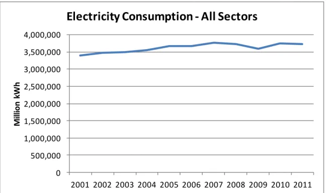
remained approximately static. Total electricity consumption has steadily increased, rising by 9% over the decade, save for a decline 2008-2009 (Figure 7). The rapid shift to gas has been facilitated by the fact that the US gas fuelled generators were previously operating at very low capacity factors4; Hultman et al (2011) report that 35% of capacity of combined cycle gas turbines (CCGT) was used in 2008, compared to a 30% capacity factor for open cycle gas turbines (OCGT) and 70% for coal plant. As such the US energy system has been able to substantially fuel switch and increase gas consumption in advance of the

construction of new plant. For comparison, in 2010 CCGT plants operated in the UK at a 61% capacity factor, down from a peak of 69% in 2008 due to recent capacity additions, and coal plants at just 41% (DECC 2011).

Figure 6 Electricity generation by fuel source

4

Capacity factor is defined by the EIA as the ratio of the electrical energy produced by a power plant for the period of time considered, to the electrical energy that could have been produced at continuous full power operation during the same period. Load factor is often used synonymously for example in the DECC Digest of UK Energy Statistics.

(11)

10

Figure 7 Electricity consumption – all sectors

A breakdown of natural gas consumption illustrates how the power sector has been the dominant source of growth in gas consumption (Figure 8). This trend began before both the large-scale production of shale gas and the recent price crash, and may therefore have other determinants. Regulations to address SO2, NOx and mercury emissions, in addition to

cooling water and ash disposal, have also contributed to the relative preference for new investments in gas generating capacity over coal (Elmquist 2012; US EPA OAR 2012). For instance, in 2010 2,200MW of new gas fired capacity came on stream, representing 84% of net new capacity added to the US grid; the same year witnessed 585MW and 636MW net of coal and oil plant respectively being retired (EIA 2012c; table 1.4).

This trend is expected to continue in the future, with more than twice as much new planned capacity for gas in 2011 and 2012 than coal, and very little coal capacity to be added to the US grid beyond 2013 (EIA 2012c; Table 1.5). As a result, the proportion of electricity

generated by natural gas is expected to increase further, from 24% to 28% by 2035, under the AEO Reference case, despite the share from renewables growing from 10% to 15% (EIA 2012g). Electricity generation from coal is lower in all of the AEO scenarios, however, a small number of the scenarios envisage absolute increases in power generation from coal by 2035 if economic growth is high, gas recovery is low or trends in the price of coal reverse.

0 500,000 1,000,000 1,500,000 2,000,000 2,500,000 3,000,000 3,500,000 4,000,000

2001 2002 2003 2004 2005 2006 2007 2008 2009 2010 2011

M

ill

ion

kW

h

(12)

11

Figure 8 Natural gas consumption by sector

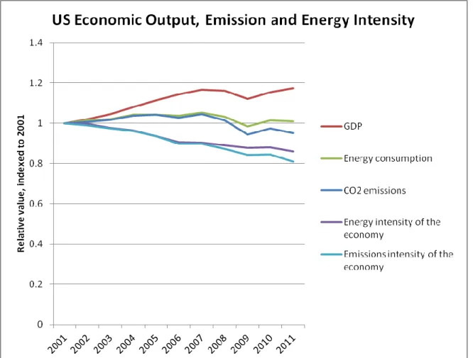
During the last decade the US economy has continuously reduced its emissions intensity of economic activity. Simultaneously, the structural shift towards a service based economy and increased efficiency have reduced the energy intensity of economic activity. These relative changes are illustrated in Figure 9. A separation of emissions intensity and energy intensity from 2007 onwards can be discerned that might be associated with changes in electricity generation and reductions in wholesale gas prices (the divergence of purple and sky blue lines below).

0 1000000 2000000 3000000 4000000 5000000 6000000 7000000 8000000

2001 2002 2003 2004 2005 2006 2007 2008 2009 2010 2011

A

b

solut

e

Co

n

su

m

p

tion

(M

M

cf)

Natural Gas Consumption by Sector

Residential Commercial Industrial Electricity

(13)

12

Figure 9 US Energy and emissions intensity trends

The outlook for future price and resource trends is somewhat uncertain, indeed the EIA has recently reported that it expects the trends in gas prices and coal consumption to reverse during 2012 (EIA 2012f). This is expected to result in a 2.8% increase in emissions in 2013. Estimates of Technically Recoverable Resources (TRR) for US shale wells have also been substantially revised down in the 2012 AEO against the 2011 AEO as new geological and well productivity data have become available. The total shale gas TRR has fallen from 847tcf to 482tcf (Table 14, p57 of AEO 2012). The largest absolute reductions relate to the

Appalachian (441tcf to 187tcf), Arkoma (54tcf to 27tcf) and Permian (67tcf to 27tcf) basins, whilst Western Gulf basin estimate has nearly trebled from 21tcf to 59 tcf. However, due to the economic considerations that determine actual production from TRRs, the overall future production expectation is itself highly uncertain. The AEO therefore considers a range of possible scenarios for Expected Ultimate Recovery (EUR) alongside TRR. Anticipated production in 2035 varies from 9.7tcf in the lowest case to 20.5tcf in the highest with the Reference scenario including 13.6tcf of shale gas (Table 19 of AEO, p62). This is against 2011 production of approximately 7.3tcf. Nevertheless, these volumes are all of a sufficient scale to be internationally relevant and in all cases the EIA anticipates the US to be a net exporter of gas in 2035. This will have ramifications for producers and consumers of gas and coal internationally.

(14)

13

4 Trends in the international trade of US coal

As noted previously, climate change is an issue of absolute and not relative emissions. Consequently, if a shift from coal to gas is to contribute to climate mitigation, the displaced coal must not be burned elsewhere within the US economy or overseas.

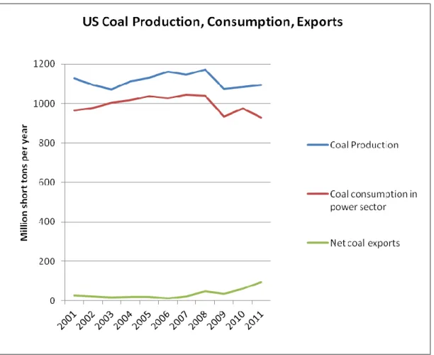
In considering the repercussions for coal production of increasing shale gas extraction, the first statistics of interest are total coal production, as displayed below. It can be seen that there was a decline associated with the economic downturn but a subsequent stabilisation and then upturn in recent years. Absolute consumption in the power sector shows a similar trajectory but with a marked divergence in 2011. The ultimate fate of this displaced coal consumption must be accounted for if the role of shale gas in mitigation is to be

understood.

Figure 10 US coal production, consumption and export

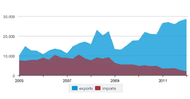
As can be seen from the figure above, the net US trade position for coal has changed substantially in the last five years. Figure 11, below, disaggregates this data to provide greater clarity on how US coal imports and exports are changing. Coal imports to the US have declined continuously since 2008 whilst exports have risen markedly5. Latest data indicate that just 2 million tons of coal was imported to the US in the first quarter of 2012,

5_{The graph below illustrates data on a quarterly rather than annual basis which must be borne in mind when}

(15)

14 down 25% from the last quarter of 2011 (EIA 2012e). Against this, gross quarterly exports rose to 28.6 million tons, indicating a net export of over 26 million tons of coal.

Figure 11 US coal exports and imports 2005 to 2012

The market for this US coal is increasingly seen to be Europe and Asia (EIA 2012d). These two regions together make up 76% of US coal exports and have shown rapid growth since 2009; for example, UK imports of US coal rose to 7 million tons in 2011 and the Netherlands rose to 11 million tons. The EIA (2012e) identifies general upward trends in coal use abroad and disruptions to supply in Australia, Indonesia and Colombia, making the US an attractive source. Within Europe, rising gas spot prices in combination with low permit prices in the EU ETS meant that there was a substantial incentive to generate electricity from coal plants rather than gas. Bloomberg Industries estimates that in the second quarter of 2012, European coal fired plants returned a profit of €16.3 per MWh, up from €9 a year earlier, whilst gas plants only just broke even (Katakey et al. 2012).

(16)

15

Figure 12 Destination of US coal exports, Source: US Energy Information Administration (2012)

5 Changes in US CO

2

emissions

US CO2 emissions from energy, excluding those from international aviation and shipping,

have declined 8.6% from a peak in 2005, the equivalent of 1.4% per annum over this period. Over the same period annual emissions from coal have declined 308Mt (14%), whilst gas increased 121Mt (10%) in 2011. With additional reductions in oil consumption, total fossil fuel emissions in 2011 were 516MtCO2 lower than in 2005.

Figure 13 US CO2 emissions from energy by fuel source

(17)

16 These trends cannot be readily dissociated from changes in economic activity. There was a marked dip due to the 2008-2009 downturn, but it is notable that emissions fell again 2011. This fall was in part due to a slight reduction in total electricity generation in 2010-2011 and increases in absolute quantities of hydro and wind generated electricity6. The EIA expect the divergence of sectoral emissions growth, from coal to gas, to intensify further in 2012, before stronger economic growth in 2013 will lead to increases emissions across the board. However, there are unmistakeable differences between trends in energy sources as Figure 14 below illustrates.

Figure 14 Recent changes in energy related CO2 emissions

There is sufficient US data to provide a provisional estimate of domestic CO2 emissions

reductions attributable to the displacement of coal by gas in electricity generation. The most up-to-date, but still provisional, data for shale gas production have been derived from submissions of EIA-23 forms presented in the U.S. Crude Oil, Natural Gas, and Natural Gas Liquids Proved Reserves report (EIA 2012g). It is assumed in our analysis that figures in Table 3 of EIA 2012g are recorded as “gross withdrawals” i.e. gas volume before the removal of non-hydrocarbon gases and losses from processing. These have been converted to dry gas production figures (i.e. gas fit for transmission, distribution and combustion) by assuming losses at the mean rate for all gas sources derived from the annual national figures in the August 2012 Monthly Energy Review (EIA 2012c). Based on these assumptions, shale gas production grew 48% from 2008 to 2009 and again from 2009 to 2010. To estimate a figure

6

This is discussed further on page 19, see also (EIA 2012c).

Forecast

-15% -12% -9% -6% -3% 0% 3% 6% 9%

2010 2011 2012 2013

U.S. Energy-Related Carbon Dioxide Emissions

annual growth

All fossil fuels Coal Petroleum Natural gas

(18)

17 for 2011 production, growth of 40% from 2010 is assumed. The resulting amount is in

accordance with the estimates illustrated in Figure 56 of the most recent AEO (EIA 2012a, p61).

Building on these estimates two simple methods of calculating avoided emissions due to fuel switching are described below. The first reviews the relative emissions intensities of US generating stations and assumes that all shale gas produced substitutes for coal. This provides a theoretical upper bound for avoided emissions. The second method takes a base case of a static fuel mix and deducts actual emissions from electricity generation as a sectoral whole. This method allows for shale gas to substitute for other sources of gas.

5.1 Method 1: Relative efficiencies of US power stations

Assuming that all ‘new’ shale gas production is combusted in marginal electricity generating powerplants (CCGTs operating at 45.9% efficiency, Hultman et al. 2011, Table 5) then it is possible to estimate both the emissions from the combustion of the gas and the anticipated quantity of electricity generated. If this electricity is assumed to have otherwise been generated by average US coal powerplant (33.9% efficiency, Hultman et al. 2011) then an estimate of potential CO2 emissions avoided is possible, as well as the equivalent mass of

coal not combusted. These calculations are presented below.

Table 1 Calculation of direct fuel switching emissions reductions

There are a number of points to note from this analysis. Firstly, a coal to shale gas switch in electricity generation may at most have led to domestic US emissions reductions of

580MtCO2 in 2011; this is ~10% of total US fossil fuel CO2 emissions and the same order of

magnitude to the total reduction in energy emissions from the 2005 peak. However, the estimated volume of shale gas produced in 2011 is only slightly lower than the total volume of gas burned in electricity production. Therefore, in combination with the trends illustrated in Figure 3, it is reasonable to conclude that other gas imports, as well as coal, are being displaced in the power sector, or that shale gas is also being used in other sectors such as industry and domestic heating.

Similarly, the fuel switch estimated here is equivalent to 44% of 2011 coal consumption. Although 2011 had relatively low coal consumption, it is still comparable to the highest recent year (2007, 1045 million short tons burned in power sector). As a result, the quantity

Year

Gross Withdrawals from Shale Gas (MMcf)

Emissions from shale gas combustion (MtCO2)

Potential Electricity from shale gas (TWh)

Equiv coal energy input for same electricity (TWh)

Equiv emissions from coal (MtCO2)

Equiv mass coal (Million short tons)

Equiv Emissions avoided (MtCO2)

2008 1,663,878 96 227 669 227 98 131

2009 2,460,453 141 336 989 335 145 194

2010 4,286,792 246 585 1,724 584 253 338

2011 7,355,087 422 1,004 2,957 1,002 435 580

For comparison, 2010 US total figures

Total gas production (MMcf)

Total gas CO2 (Mtonnes)

Total electricity consumption (TWh)

Total gas consumption for electricity (MMcf)

Total coal CO2 (MtCO2)

Power sector coal consumption (Mst)

Total fossil fuel emissions (MtCO2) 2010 21,577,211 1,265 3,755 7,680,330 1,874 975 5,601

(19)

18 of avoided emissions due to fuel switching calculated here is almost certainly an

overestimate. Caveats

This analysis does not account for:

 Anything other than the availability of shale gas driving or supplying the fuel switch from coal to gas e.g. climate policies such as the Regional Greenhouse Gas Initiative covering 10 states on the eastern seaboard (http://www.rggi.org/).

 Fugitive methane emissions of either fuel at any point in the electricity supply

 Other lifecycle energy consumption and CO2 impacts

 Changes in demand for electricity resulting from relative price changes

 The actual heat content of coal and composition of coal displaced / exported. Heat content of coal by unit mass varies substantially by coal type, a uniform central figure of 0.33884 kgCO2e/kWh (DEFRA 2010) is used here.

5.2 Method 2: Power sector fuel switching taken in aggregate

Alternatively, emissions reductions can be estimated from an assumed baseline, in the manner of carbon offset calculations performed under the UNFCCC Clean Development Mechanism. In effect we assume that the same quantity of electricity would have been generated in the years after shale gas availability (2008-2011) but with the fuel mix in the period before shale gas availability (2005-2007) and compare emissions output.

Emissions intensity of US electricity production had been stable from 2001 to 2005 at around 660 to 670 tonnes CO2/GWh, with a slight fall to approximately 644 tonnes

CO2/GWh in 2006 and 2007. Further year on year reductions then occurred from 2007

onwards.

(20)

19 If we assume a baseline of the grid emissions factor averaged over the three years prior to large scale shale gas production (2005 to 2007) is extended 2008 to 2011, then we have a counterfactual emissions trajectory for electricity generation. Table 2 indicates that

emissions would remain at approximately 2400 MtCO2 per annum if electricity consumption

was as recorded but the fuel mix remained static. Subtracting actual emissions from this baseline provides an estimate of emissions avoided in the power sector over this period presented as the shaded area in Figure 16 below.

Table 2 Grid emissions reductions from baseline

Figure 16 Avoided emissions, baseline method

The resulting potential avoided emissions are calculated to be between 50 and 250 MtCO2

per annum, rising significantly over this period. For 2011, this is less than half the headline figure of 516Mt reduction 2005 to 2011 cited for the US economy as a whole. Clearly, not all of the reduction in US emission output has occurred within the power sector, reductions in other sectors, such as domestic heating and transport, accounting for the other half.

2005 2006 2007 2008 2009 2010 2011 CO2 from electricity generation (MtCO2) 2,417 2,359 2,426 2,374 2,159 2,271 2,166 Consumption of electricity (GWh) 3,660,969 3,669,919 3,764,561 3,732,962 3,596,865 3,754,493 3,726,163 Emissions intensity of electricity (tCO2/GWh) 660 643 644 636 600 605 581 Mean emissions intensity electricty

2005-2007 (tCO2/GWh) 649

Baseline emissions power sector (MtCO2) 2,423 2,335 2,437 2,419 Avoided emissions in power sector (MtCO2) 50 176 166 253 Potential max emissions reduction

coal to gas switch in electricity (MtCO2) 131 194 338 580 Potential Electricity from shale gas (GWh) 227,130 335,868 585,175 1,004,018

(21)

20 This method implicitly accounts for the substitution of gas imports and domestic gas

production unlike that in Section 5.1. However, potential emissions reductions calculated for either method do not account for any substitution by shale gas in sectors other than electricity e.g. in industrial processes.

The estimates shown in Table 2 are less than the emissions reductions calculated by the method in Section 5.1, suggesting that it would be physically possible for shale gas price effects to account for all of the fuel switch were it substituting for coal alone. However, this does not appear to be the case from the trends in gas imports shown in Figure 4, above, and electricity generation from oil outlined in Table 3, below.

Potentially avoided emissions are calculated for the grid as a whole so large scale changes in electricity generation from renewable or nuclear sources are also captured. As outlined in Section 3.1, the changes in these sectors are smaller than the shift from coal to gas

combustion. Table 3 (below, and reproduced for clarity on p28) quantifies this shift in terms of the difference between electricity generated in recent years and a 2005-2007 baseline. Reductions are also seen in petroleum consumption, with very small increases in nuclear and hydro when summed across the period 2008-2011 to account for inter-annual variation. The cumulative increase in generation from gas is more than double the increase from wind, although the increase from wind is itself substantial.

Table 3 Trends in generation by fuel source (Data: EIA 2012 Monthly Energy Review Table 7.2b, red indicates reduction, only major fuel sources shown, collectively 99% of generation)

As Figure 3 describes, imports and conventional domestic production of natural gas have been declining during this period, so it is not unreasonable to assume that the increase in shale gas production has contributed to this shift. However, it is important to note that Method 2 does not isolate the price effect of shale on the power sector, nor any

simultaneous change in emissions in the non-power sector e.g. chemical and manufacturing industry.

In conclusion, this method is less likely to overestimate potential avoided emissions than the direct fuel switch method presented in Section 5.1 by allowing for internal substitution in the gas market. However, it captures the power sector as a whole, within which the growth in wind generation and the impact of other policies are significant.

Electricity Net Generation From Coal, Electric Power Sector Coal 2005-2007 baseline generation Electricity Net Generation From Petroleum, Electric Power Sector Petroleum 2005-2007 baseline generation Electricity Net Generation From Natural Gas, Electric Power Sector

Natural Gas 2005-2007 baseline generation Electricity Net Generation From Nuclear Electric Power, Electric Power Sector Nuclear 2005-2007 baseline generation Electricity Net Generation From Hydroelectric Power, Electric Power Sector Hydro 2005-2007 baseline generation Electricity Net Generation From Wind, Electric Power Sector Wind 2005-2007 baseline generation (Million Kilowatthours) (Million Kilowatthours) (Million Kilowatthours) (Million Kilowatthours) (Million Kilowatthours) (Million Kilowatthours) (Million Kilowatthours) (Million Kilowatthours) (Million Kilowatthours) (Million Kilowatthours) (Million Kilowatthours) (Million Kilowatthours) 2005 Total 1,992,054 1,986,727 116,482 79,165 683,829 744,333 781,986 791,877 267,040 266,379 17,811 26,283 2006 Total 1,969,737 59,708 734,417 787,219 286,254 26,589

2007 Total 1,998,390 61,306 814,752 806,425 245,843 34,450 2008 Total 1,968,838 - 17,890 42,881 - 36,284 802,372 58,039 806,208 14,332 253,096 - 13,283 55,363 29,080 2009 Total 1,741,123 - 245,604 35,811 - 43,354 841,006 96,673 798,855 6,978 271,506 5,127 73,886 47,603 2010 Total 1,827,738 - 158,990 34,679 - 44,487 901,389 157,057 806,968 15,092 258,455 - 7,924 94,636 68,353 2011 Total 1,714,870 - 271,857 26,223 - 52,942 930,568 186,236 790,225 - 1,652 323,141 56,762 119,704 93,421 Cumulative

increase 2008-2011 - 694,340 - 177,068 498,005 34,750 40,682 238,456 Change against baseline Change against baseline Change against baseline Change against baseline Change against baseline Change against baseline Year

(22)

21

5.3 Econometric approaches to estimating substitution

A further means of calculating the scale of the shift from coal to gas is to estimate the short term price elasticity of fuel substitution, i.e. the comparative change in consumption of a fuel expected for a given price change. Econometric models are used to identify statistically significant relationships in data sets and estimate elasticities. These values can then be used to make inferences about other parts of the economy where the fuel switching relationship is unclear. The EIA (2012b) has used this method to analyse price and consumption data, at a fine spatial and temporal scale, within the US power sector. It was found that relationships are, on the whole, weak due to a range of confounding but important factors such as

available capacity, technical characteristics of generators, and environmental regulations. The EIA (2012b) found substantial regional variations with the elasticity estimates most robust for the Southeastern states but insignificant for Texas and the Midwest. However, this method is recognised within the energy economics literature and offers a causative insight that the methods 1 and 2 above do not.

Two recent studies are worth noting. Lu et al. (2012) use a regional econometric model calibrated with data from 2005-2010 to analyse the reduction in emissions from 2008 to 2009. They estimate that just over half of the observed decrease in emissions from the power sector in this period (215 MtCO2) could be attributed to the reduction in gas price,

the remainder predominantly due to the economic downturn.

Afsah and Salcito (2012), using the EIA’s mean national estimate of the substitution

elasticity of coal to gas of 0.14 (2012b), calculate that coal’s relative price increase of 109% from 2006 to 2011 could have increased relative gas consumption by 15%, equivalent to 89 million MWh of electricity displacement. They note that this figure is just 35% of the total reduction in coal fired electricity generation in this period. The remaining reduction in coal burned in the power sector is attributed to regulations, energy efficiency/demand

management, improving cost-competitiveness of renewables, the recession and NGO campaigns. In total they estimate that 50Mt of CO2 reduction from 2006 to 2011 was due to

price effects, including the small shift from oil to gas in the power sector.

In conclusion, econometric methods suggest a means of identifying price effects within a system of multiple policy and economic drivers, however a full appraisal of these methods is beyond the scope of this report.

6 Impact on CO

2

Emissions Outside of US

If shale gas has caused displacement of US coal consumption in the power sector then emissions are only reduced in net terms if that coal is not burned elsewhere or at another time. Coal exported to countries with growing economies and without an effective

emissions cap is likely to represent an increase in emissions.

Exports of coal to uncapped economies with growing demand for energy are assumed to contribute directly to increased emissions as they serve to reduce effective fuel prices and thereby increase demand. This case is stronger against a background of rising fuel

(23)

22 that despite a small reduction in oil and gas consumption from 2008 to 2009, there is no long term indication of demand for coal or gas abating. Indeed data from the BP Statistical Review (2012) shows that coal is the fastest growing fossil fuel in recent years, increasing by an average of 3.8% per annum 2005 to 2011 resulting in a total increase of 25% over this period.

Figure 17 Global energy consumption, data from BP Statistical Review (2012)

It is therefore reasonable to consider emissions from the non-US combustion of displaced US coal as part of the consequences of fuel switching in the US power sector. Wherever displaced US coal is combusted, in the absence of polices to force fossil fuel substitution there will be an absolute increase in global emissions and hence a reduced probability of avoiding the 2°C characterisation of dangerous climate change.

Table 4 estimates the displaced volume of US coal by deducting a baseline average of mean exports in the period 2005-2007 from total net exports in the period 2008 to 2011. Whether or not these exports are entirely due to shale gas or wind displacing coal from the US power sector cannot be demonstrated in this way. However, the calculations in Section 5 show that the mass of coal exported is less than the potential for displacement in the power sector; a position supported by the timing of respective emissions and production trends.

Comparing the scale of avoided emissions due to fuel switching in the power sector to the emissions implicit in coal exports suggests that more than half of the potential emissions avoided may be displaced outside the US. We suggest that 75 million short tons of coal exported from the US in 2011 may be due to displacement, implicitly adding 154 MtCO2 to

(24)

23

Table 4 US Grid emissions reductions in comparison to coal exports

Therefore, net avoided emissions due to fuel switching on the US grid in 2011 might better be regarded as approximately 100 MtCO2. Conversely, if this quantity of displaced emissions

is added to the US CO2 output from fossil fuel combustion, see Figure 13, the reduction from

the peak in 2005 would be 362 MtCO2 i.e. a 6% change over this whole period or less than

1% per annum. Totalling the quantity of implicit emissions exported over the period 2008 to 2011 suggests that more than half (52%) of the potential avoided emissions from the

baseline are lost; 645 MtCO2 avoided, in comparison to 338 MtCO2 exported.

It is important to note that these calculations are dependent upon many assumptions not least that avoided emissions are calculated from a counterfactual baseline. It is also taken that coal displaced but not exported is not burned at any point in future. Finally, it is worth reiterating that it cannot be assumed that the price effect of shale gas availability is

responsible for these changes.

The latest data available show the trend in exports to be increasing and also the destination of exports (Table 5), which may have some bearing on the climatic implications due to consuming nations’ climate policy framework.

Table 5 Coal exports and implicit emissions7

In the first quarter of 2012 more than half of US coal exports were to Europe and therefore almost certainly included within the EU ETS. As this is a cap and trade system, the total emissions over the period of its operation should not be breached and there should be no net global increase due to this import, unless this results in secondary changes in the trade of other fuel sources. One might expect displacement of other fuel sources within Europe, for instance away from indigenous fuels or coal and gas imported from other countries. This

7_{Historic monthly export data do not show substantial, consistent, seasonal differences so the annual}

extrapolation appears reasonable (EIA 2012c).

2005 2006 2007 2008 2009 2010 2011

Aggregate 2008-2011

Net coal exports (Mst) 20 13 23 47 36 62 94

Mean net coal exports 2005-2007 (Mst) 19

Additional exports due to displaced

production (Mst) 29 18 44 75 165

Implicit coal emission exported (MtCO2) 58 36 89 154 338

Avoided emissions in power sector

due to fuel switch (MtCO2) 50 176 166 253 645

Proportion of avoided emissions

represented by displaced coal (%) 118% 21% 54% 61% 52%

Net avoided emissions due to fuel

switch and coal displacement (MtCO2) -9 140 77 99 308

Annual equivalent Destination Mass Coal (short tons) Emissions (MtCO2) (MtCO2)

To Europe 16,359,777 37 149

To non-EU 12,281,921 28 112

Total 28,641,698 65 260

(25)

24 creates the potential for secondary effects, for instance on the prices of fuels traded with Europe such as Australasian coal or LNG from the Arabian Gulf.

Further, the EU ETS is over supplied with emissions permits primarily as a result of the economic downturn. Although this policy instrument was intended to drive decarbonisation of the power sector, the price of EUAs has been persistently low and is expected to remain so throughout the third phase (2013 to 2020) as the excess from the second phase will be carried over. Presently there appears to be little or no abatement occurring in Europe as a result of the ETS (Morris 2012). Without a radical modification to the EU ETS imports of coal are likely to add to emissions overall and act as a disincentive to investment in lower

emissions infrastructure.

Ultimately, even if the imported coal is combusted in a nation or region with emission caps more stringent than the EU, of which none exists at present, there are very likely to be levels of second-order displacement that negate any mitigation benefits. Provided normal levels of profit can be realised from the extraction of fossil fuels, it is difficult to envisage a market-led energy system not extracting and combusting such fuel. Given the global market for fossil fuels is growing and that global economic growth remains dependent on access to such fossil fuels, extraction of a new fossil fuel source is likely to depress overall fossil fuel prices and by definition increase demand i.e. catalyse an increase in absolute emissions. In this regard, and in the absence of meaningful emission caps, shale gas extraction within a market-based energy system will lead to an absolute increase in emissions.

(26)

25

7 Conclusions

This report has explored the emissions consequences of fuel switching in the US energy system using two simple methodologies. The analysis presented is conditional upon its internal assumptions, but provides an indication of the scale of potential changes due to increases in shale gas and wind power. It suggests that emissions avoided due to fuel switching in the US power sector may be up to 50% of the total reduction in US energy system CO2 emission since their peak in 2005. As discussed in our previous work (Broderick

et al. 2011), without a meaningful cap on global carbon emissions, the exploitation of new shale gas reserves is likely to increase total emissions. For this not to be the case,

consumption of displaced fuels must be reduced globally and remain suppressed

indefinitely; in effect, displaced coal must stay in the ground. Neither the availability of shale gas, nor other policies that transfer power generation away from coal, guarantee this in and of themselves. However, renewable capacity does not directly release carbon dioxide emissions during generation.

Within national boundaries the suppression of gas prices through shale gas availability is a plausible causative mechanism for a proportion of avoided emissions, but the research conducted here has not isolated the proportion of fuel switching due to this effect. Other studies note that between 35% and 50% of the difference between US peak and present power sector emissions may be due to shale gas price effects. The interactions with other US climate and energy policies including cap and trade regulations such as the RGGI have not been investigated.

Whilst there appears to have been a recent shift in US electricity generation that may have realised localised CO2 emissions reductions, it is not clear that there have been substantial

net reductions globally. The calculations presented here suggest that more than half of the potential emissions avoided in the US power sector may actually have been exported as coal. Totalling the quantity of implicit emissions exported over the period 2008 to 2011 suggests that approximately 340 MtCO2 of the 650 MtCO2 of emissions avoided may be

added elsewhere.

Demand for energy is increasing globally and if this continues to be supplied by fossil fuels then dangerous interference with the climate is increasingly likely. Were an abrupt, internationally simultaneous, fuel switch from coal to gas to occur, the remaining safe carbon budget may be consumed less quickly. In the ‘real world’ these conditions are unlikely to coincide. The analysis presented in this report suggests that localised fuel switching may not in fact realise the scale of benefits promised by simple comparison of emissions intensity statistics.

Despite downwards revisions to estimates of unconventional gas resources it is likely that this issue will continue to be of relevance to climate policy. It remains to be seen whether the recent trends within the US persist and what the consequences of unconventional gas production outside of the US will be. Further quantitative research into energy system changes is needed if unconventional gas is to be developed globally and the emissions implications understood.

(27)

26

8 References

Afsah, S. & Salcito, K., 2012. Shale Gas And The Overhyping Of Its CO2 Reductions. Available at: http://thinkprogress.org/climate/2012/08/07/651821/shale-gas-and-the-fairy-tale-of-its-co2-reductions/ [Accessed August 30, 2012].

BP, 2012. Statistical Review of World Energy 2012 | BP, Available at:

http://www.bp.com/sectionbodycopy.do?categoryId=7500&contentId=7068481 [Accessed September 20, 2012].

Broderick, J. et al., 2011. Shale gas: an updated assessment of environmental and climate change impacts, Tyndall Centre for Climate Change Research. Available at:

http://www.tyndall.manchester.ac.uk/public/Tyndall_shale_update_2011_report_su mmary.pdf.

DECC, 2011. Digest of UK Energy Statistics,

EIA, 2012a. Annual Energy Outlook 2012, US Energy Information Administration. Available at: http://www.eia.gov/forecasts/aeo/.

EIA, 2011. Electric Power Annual 2010, US Energy Information Administration. Available at: http://www.eia.gov/electricity/annual/pdf/epa.pdf.

EIA, 2012b. Fuel Competition in Power Generation and Elasticities of Substitution, US Energy Information Administration. Available at:

http://www.eia.gov/analysis/studies/fuelelasticities/.

EIA, 2012c. Monthly Energy Review - August 2012, US Energy Information Administration. Available at: http://www.eia.gov/totalenergy/data/monthly/#summary.

EIA, 2012d. Most U.S. coal exports went to European and Asian markets in 2011. EIA. Available at: http://www.eia.gov/todayinenergy/detail.cfm?id=6750 [Accessed July 4, 2012].

EIA, 2012e. Quarterly Coal Report June 2012, US Energy Information Administration. Available at: http://www.eia.gov/coal/production/quarterly/.

EIA, 2012f. Short-Term Energy Outlook, US Energy Information Administration. Available at: http://www.eia.gov/forecasts/steo/report/.

EIA, 2012g. U.S. Crude Oil, Natural Gas, and Natural Gas Liquids Proved Reserves, 2010, US Energy Information Administration. Available at:

http://www.eia.gov/naturalgas/crudeoilreserves/pdf/uscrudeoil.pdf.

Elmquist, S., 2012. Appalachian Coal Fights for Survival on Shale Boom: Commodities. Bloomberg. Available at:

http://www.bloomberg.com/news/2012-03-21/appalachian-coal-fights-for-survival-on-shale-boom-commodities.html [Accessed July 5, 2012].

(28)

27 Harrabin, R., 2012. Anger over agency’s shale report. BBC. Available at:

http://www.bbc.co.uk/news/science-environment-18236535 [Accessed September 22, 2012].

Helm, D., 2011. The peak oil brigade is leading us into bad policymaking on energy. The Guardian. Available at:

http://www.guardian.co.uk/commentisfree/2011/oct/18/energy-price-volatility-policy-fossil-fuels [Accessed July 4, 2012].

Hultman, N. et al., 2011. The greenhouse impact of unconventional gas for electricity generation. Environmental Research Letters, 6(4), p.044008.

IEA, 2011. World Energy Outlook 2011 Special Report - Are we entering a golden age of gas?, Paris, France. Available at: http://www.worldenergyoutlook.org/goldenageofgas/. Katakey, R., Singh, R.K. & Morison, R., 2012. Europe Burns Coal Fastest Since 2006 in Boost

for US Energy. Bloomberg.

Kuhn, M. & Umbach, F., 2011. Strategic perspectives of unconventional gas: A game changer with implication for the EU’s energy security, London: European Centre for Energy and Resource Security.

Lovelock, J., 2012. James Lovelock on shale gas and the problem with “greens.” The Guardian. Available at:

http://www.guardian.co.uk/environment/blog/2012/jun/15/james-lovelock-fracking-greens-climate [Accessed July 5, 2012].

Lu, X., Salovaara, J. & McElroy, M.B., 2012. Implications of the Recent Reductions in Natural Gas Prices for Emissions of CO2 from the US Power Sector. Environmental Science & Technology, 46(5), pp.3014–3021.

Morris, D., 2012. Losing the Lead. The 2012 Environmental Outlook for the EU ETS, London: Sandbag. Available at:

http://www.sandbag.org.uk/site_media/pdfs/reports/Losing_the_lead_modified_3. 8.2012.pdf.

Rogers, H., 2011. Shale gas—the unfolding story. Oxford Review of Economic Policy, 27(1), pp.117 –143.

The Economist, 2012. Frack On; People should worry less about fracking, and more about carbon. Available at: http://www.economist.com/node/21540275 [Accessed June 27, 2012].

US EPA OAR, 2012. Cross-State Air Pollution Rule (CSAPR). Available at: http://www.epa.gov/airtransport/ [Accessed July 5, 2012].

(29)

28

Reproduction of Table 3 Trends in generation by fuel source

Data: EIA 2012 Monthly Energy Review Table 7.2b, red indicates reduction, only major fuel sources shown, collectively 99% of generation

El e ct ri ci ty N e t G e n e ra ti o n Fr o m C o al , El e ct ri c Po w e r Se ct o r C o al 2 00 5-20 07 b ase li n e ge n e ra ti o n El e ct ri ci ty N e t G e n e ra ti o n Fr o m Pe tr o le u m , El e ct ri c Po w e r Se ct o r Pe tr o le u m 2 00 5-20 07 b ase li n e ge n e ra ti o n El e ct ri ci ty N e t G e n e ra ti o n Fr o m N at u ra l G as, E le ct ri c Po w e r Se ct o r N at u ra l G as 20 05 -20 07 b ase li n e ge n e ra ti o n El e ct ri ci ty N e t G e n e ra ti o n Fr o m N u cl e ar El e ct ri c Po w e r, El e ct ri c Po w e r Se ct o r N u cl e ar 2 00 5-20 07 b ase li n e ge n e ra ti o n El e ct ri ci ty N e t G e n e ra ti o n Fr o m H yd ro e le ct ri c Po w e r, E le ct ri c Po w e r Se ct o r H yd ro 2 00 5-20 07 b ase li n e ge n e ra ti o n El e ct ri ci ty N e t G e n e ra ti o n Fr o m W in d , El e ct ri c Po w e r Se ct o r W in d 2 00 5-20 07 b ase li n e ge n e ra ti o n (M il li o n K il o w at th o u rs) (M il li o n K il o w at th o u rs) (M il li o n K il o w at th o u rs) (M il li o n K il o w at th o u rs) (M il li o n K il o w at th o u rs) (M il li o n K il o w at th o u rs) (M il li o n K il o w at th o u rs) (M il li o n K il o w at th o u rs) (M il li o n K il o w at th o u rs) (M il li o n K il o w at th o u rs) (M il li o n K il o w at th o u rs) (M il li o n K il o w at th o u rs) 2005 To ta l 1 ,9 92 ,0 54 1 ,9 86 ,7 27 1 16 ,4 82 7 9, 16 5 6 83 ,8 29 7 44 ,3 33 7 81 ,9 86 7 91 ,8 77 2 67 ,0 40 2 66 ,3 79 1 7, 81 1 2 6, 28 3 2006 To ta l 1 ,9 69 ,7 37 5 9, 70 8 7 34 ,4 17 7 87 ,2 19 2 86 ,2 54 2 6, 58 9 2007 To ta l 1 ,9 98 ,3 90 6 1, 30 6 8 14 ,7 52 8 06 ,4 25 2 45 ,8 43 3 4, 45 0 2008 To ta l 1 ,9 68 ,8 38 - 1 7, 89 0 4 2, 88 1 - 3 6, 28 4 8 02 ,3 72 5 8, 03 9 8 06 ,2 08 1 4, 33 2 2 53 ,0 96 - 1 3, 28 3 5 5, 36 3 2 9, 08 0 2009 To ta l 1 ,7 41 ,1 23 - 2 45 ,6 04 3 5, 81 1 - 4 3, 35 4 8 41 ,0 06 9 6, 67 3 7 98 ,8 55 6 ,9 78 2 71 ,5 06 5 ,1 27 7 3, 88 6 4 7, 60 3 2010 To ta l 1 ,8 27 ,7 38 - 1 58 ,9 90 3 4, 67 9 - 4 4, 48 7 9 01 ,3 89 1 57 ,0 57 8 06 ,9 68 1 5, 09 2 2 58 ,4 55 - 7 ,9 24 9 4, 63 6 6 8, 35 3 2011 To ta l 1 ,7 14 ,8 70 - 2 71 ,8 57 2 6, 22 3 - 5 2, 94 2 9 30 ,5 68 1 86 ,2 36 7 90 ,2 25 - 1 ,6 52 3 23 ,1 41 5 6, 76 2 1 19 ,7 04 9 3, 42 1 C u m u la ti ve in cr ea se 2 00 8-20 11 69 4, 34 0 - 17 7, 06 8 - 49 8, 00 5 34 ,7 50 40 ,6 82 23 8, 45 6 Y e ar C h a n g e a g a in st b a se li n e C h a n g e a g a in st b a se li n e C h a n g e a g a in st b a se li n e C h a n g e a g a in st b a se li n e C h a n g e a g a in st b a se li n e C h a n g e a g a in st b a se li n e