ISSN: 2278-3369
International Journal of Advances in Management and Economics Available online at: www.managementjournal.info
RESEARCH ARTICLE
Recalibration of the Lusk & Halperin Benford Screening Intervals:
The Relative FPE and FNE Jeopardy Considerations
Edward J. Lusk
1*, Michael Halperin
21The State University of New York (SUNY) at Plattsburgh, 101 Broad St.. Plattsburgh, NY, USA & Emeritus, Department of Statistics, The Wharton School 3730 Walnut St., University of Pennsylvania, Philadelphia, PA, USA.
2Director Lippincott Library of the Wharton School [Retired], 3420 Walnut St. University of Pennsylvania, Philadelphia, PA.
*Correspondence: E-mails: [email protected] or [email protected]
Abstract
Lusk & Halperin [1,2] offered a screening interval for the first digit Benford Profile that was basically founded on the usual parametric distribution that is associated with proportions. They created the precision using the wide-spanning 99thpercentile z-value. It was validated on the dataset offered by Reddy & Sebastin [3]. In this paper we offer a recalibrated screening protocol centered on the corrected Benford empirical bin-means founded only on the Empirical Distribution of additional Conforming and Non-Conforming datasets reported in the literature. We should find that, as expected, the initial Screening Interval is wider than the re-calibrated Screening Interval. This of course begs questions as to the False Negative and False Positive screening jeopardy. We present and discuss these relative error profiles in the context of the certified audit where the Benford Screenings are then used to identify Extended Procedure candidates.
Keywords: Newcomb-Benford First Digit Profiles Empirical Re-Calibration.
Introduction
The importance of the Benford screening had been documented in numerous research reports. It has been a staple in forensic studies for more than two decades [3-9]. The definitive logical proof of Newcomb’s [10] observation & Benford’s re-observation and investigations were provided by Hill [11-14]. There is no reported FPE & FNE probability inferential basis that is derivable from the population logistics for the first digit profile.
This is largely due to the nested conditional probabilities which have no discernable Bayes priors or, for that matter, conditional order effects down to the n-1st non-independent action. However, Lusk and Halperin [1] in taking advantage of the Benford’s Bin-Reported illustrations corrected the reported probabilities. Also see Cho and Gaines [15] who report the same corrections however without details as to the
computations. Lusk & Halperin then formed for this “Empirical” MLE central tendency profile the first digit profile screening intervals. This was done by creating variances formed around the z-calibration for a “wide-range” interval where they used the 99th Normal variate to form the precision controlling, of course, for the sample size per Bin rather than overall.
An illustrative example will be helpful.
Consider the “3” Bin. The
counting/realization standard deviation of Bin 3 that contained 20,229 events, for which 2,562were identified as Bin 3 events, was: 0.332589. The 99% z-variate used was 2.33. The precision for Bin 3 is: Precision1 = 2.33 [0.332589 /2,562] = 0.01531
1We elected to use the counting measures to compute
This gives the Alert-Window for the occurrences of “3” as recorded in Table 2following as:Benford corrected frequency [Bin (3)] 0.01531, or [0.111340 to 0.141960] computed as: [0.126650 0.01531]
We shall refer to this as the initial Benford Screening Intervals [IBSI]. They then tested the IBSI by scoring the 12 Non-Conforming datasets reported by Reddy and Sabastin [3].
If a particular digit of these 12 Non-Conforming datasets was not in the IBSI then that digit was scored as “Alert” otherwise “Non Alert”. There were 71 such “Alerts” of the 108 possibilities [12 × 9] giving an alert percentage of the test datasets of 65.7%. This was then the screening percentage used as the MLE cut-point for a particular dataset to be screened. In summary, if there are more than five alerts [6, 7, 8 or 9] then the dataset is scored as Non-Conforming otherwise Conforming relative to the Benford Profile. All of the technical details for this computation are reported in their initial paper cited above. This is the point of departure of this research paper.
Interest in the nature of this Benford Screening Interval has to do with identifying particular accounts in the audit context that are likely candidates for Extended Procedures [EP] investigations. This is a fundamental idea and underlies the spirt of AS2 and the current version AS5 promulgated by the PCAOB: the audit licensing arm of Sarbanes-Oxley: 2002 [PL: 107-204]. The logic is pristine: The audit is based upon on a random sample of accounts, usually sensitive accounts, which are those client accounts that affect the Current Ratio & Cash Flow from Operations. As the In-Charge cannot investigate ALL of these accounts, due to time and resource constraints, some of the sensitive accounts must be selected for EP investigation. In this case, it is recommended that all the sensitive accounts be screened using the IBSI. Those
computation of precision using the developed frequency information for large sample sizes. For example, Precision is:
𝑧 × √𝑝 × (1 − 𝑝) 𝑛
For the example above: 2.33 [(0.126650(1 0.126650))^0.5] / 2,562 = 0.01531.
accounts flagged as Non-Conforming, respecting the Benford profile, are selected as viable candidates for EP investigations such as: Confirmations: [addressing the PCAOB Management Assertions of:
Existence, Valuation& Rights, Tracing &Vouching:[addressing the PCAOB Management Assertions of: Completeness
& Occurrence and often Categorization: [addressing the PCAOB Management Assertion of: Classification]. To say the least these EP Investigations are very costly and so if care is not taken in conducting EP investigations the resource control of the audit will be lost to the detriment of all concerned.
Précis of the Research
We will: Take a set of Non-Conforming Datasets & a set of Conforming Datasets that are reported in the literature and use their empirical presentations to create central [Mean] tendencies,
Form, based upon these two profile sets, Absolute differences from the corrected Benford first digit central tendencies for each of the nine first digits,
Use these measured distances over the Non-Conforming and Conforming dataset store-form the screening intervals. Refer to this recalibration as: RBSI,
Test the two Screening Intervals, IBSI & RBSI, for their FNE and FPE screening jeopardies. This will be very important decision making information as L&H did not offer information as to the jeopardy profiles of the IBSI,
Considering the Monetary Risk of scripting wrong Audit Opinion and the high Cost of launching Extended Procedures investigations, offer a graphic and taxonomy of this Monetary Risk & EP Cost trade-off for guiding the selection of the particular Benford screening interval: IBSI or RBSI.
The Test Datasets
years. These data profiles are are available from the author for correspondence. There were 24Non-Conforming [NC] datasets that were so judged/ evaluated by the researchers reporting their results and 31Conforming datasets [C].
In creating a new set of Benford screening intervals that are empirically driven, as opposed to the statistically based screening intervals of L&H, we computed the Mean profile for the NC, n = 24 and C, n= 31 datasets. We then tested these two samples [NC & C] for non-directional comparisons respecting the Null of no difference for each of the nine first digits. Here we used the t-test assuming unequal variances as the
three standard tests for unequal variance of the SAS: JMPv. 13 Data Analysis platform:[Brown & Forsythe [16] Levene [17] and O’Brien [18] indicated that, excepting digit 4,all of the remaining eight digits had p-values lower than 0.25 for the Null of equal variance. In this case, for the mean tests, NC vs. C, there were four digits, {1, 5, 8& 9}, that had two-tailed p-values < 0.15 certainly indicative of overall profile differences between the NC & C groups. This result is particularly impressive as the inferential Power respecting the p-value was relatively Low. The Mean Profile of these datasets is presented in Table 1.
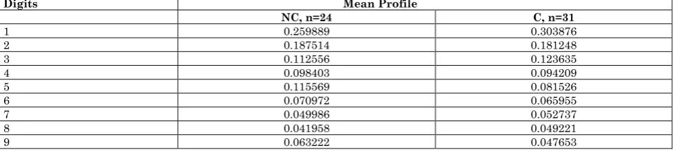
Table 1: The mean values of the first digit profiles for the non-conforming & conforming datasets Digits Mean Profile
NC, n=24 C, n=31
1 0.259889 0.303876
2 0.187514 0.181248
3 0.112556 0.123635
4 0.098403 0.094209
5 0.115569 0.081526
6 0.070972 0.065955
7 0.049986 0.052737
8 0.041958 0.049221
9 0.063222 0.047653
To be clear, the information in Table 1 shows the Mean values of the percentages, as reported in the literature, for the 24 instances of Non-Conforming datasets as reported in Col2. In Col3 are the Mean values for the 31 instances of datasets that were reported in the literature as Conforming. For example, for Digit 1 the Mean value of the 24 Non-Conforming datasets was 0.259889; the Mean for the 31 Conforming datasets was 0.303876. There difference tested to be different; has it had a non-directional p-value 0.03.
We used Table 1 as the base information to derive the modifications to the IBSI reported by L & H. Specifically, we took the information in Table 1 and formed, for each first digit, the difference between the Mean
Corrected results reported by L&H and the NC & C profiles reported in Table 1.This produced two values for each digit; one of which is the directed distance between Corrected Mean and the Mean of the NC; the other being the distance between Corrected Mean and the Mean of the C. We then took the absolute value as there is no information relative to direction or in this case: the sign of the directional difference. Then for these two relative distances we took their average so as to smooth as much as possible the symmetry of the recalibration. An example will be instructive. To elucidate the computations that were made to re-calibrate the IBSI to form the RBSI, consider the following profiling as reported in Table 2.
Table 2:
First Digits
L&H Benford Screens Empirical Profile Average Abs Diff
Re Calibrated BSI Precision Ratios LHS IBSI RHS IBSI NC, n=24 C, n=31 LHS RBSI RHS RBSI
1 0.275377 0.303001 0.259889 0.303876 0.021994 0.267195 0.311183 1.59
Consider Digit 1 as shaded and bolded in Table 2. The Corrected Benford mean Profile as reported by L&H and Cho & Gaines is found by taking the simple average of the Left Hand Side [LHS] & the Right Hand Side [RHS] of the L&H intervals. This is: 0.289189 [(0.275377 0.303001)/2]. This will be the mid-point of the recalibrated BSI which, of course, is necessary to avoid a shift-bias. The simple average of the absolute differences as found in Col6 of 0.021994 is found as follows: The absolute difference between [0.259889 and 0.289189] is0.0293; this is the non-directional distance for the Non-Conforming datasets. For the other side of the interval, which is the Conforming dataset information, we have the absolute difference between [0.303876 and 0.289189] which is 0.014687. This gives
the average as 0.021994
[(0.02390.014687)/2]. The next computation is to create the new empirical IBSI or RBSI. In the case of Digit1 this is 0.289189
0.021994 which gives:
0.267195&0.311183as reported in Col7 & Col8.
In the manner that we created there-calibration there is no reason to proffer that the transformation RBSI is isomorphic with the IBSI as created by L&H. To show that this is the case and also to give the profile information that relates to the precision expectation discussed above, we measure the precision of the two BSIs and formed the Ratio: Precision [RBSI] / Precision [IBSI]. For example for Digit1 we find: [(0.3111830.267195)/2]/[(0.3030010.27537 7)/2]which gives a ratio of 1.59 as reported in whole percent in Col9 of Table 2.
We see from these precision ratios that there is no evidence of a strict homomorphy to wit all the ratios would be the same constant, the special case of which would be 1.0, or, for that matter, an order homomorphy where all ratios would either be greater or less than unity. Also, we observe that overall the Mean/Median of the ratios over the nine digits is 0.69/0.56confirming that the IBSI is robustly slightly wider than RBSI overall.
As a final indication of the relative performance of these two screening intervals, we indexed the various theoretical
expectations: Log10(1 + 1/j); where j = 1, 2, - - -, 9 to have increments such that over 100 changes these incremental adjustments would finally arrive at the most extreme case of a digital anomaly: the Hill(1998) Lottery expectation of 1/9. For example, for the first digit 0.30103 the incremental change to finally arrive at 1/9 over 100 modifications is: [Log 10(1 + 1/1) 1/9]/100 = 0.18992%
In this case then we took these 100 datasets and tracked where the first transition point existed from the movement from Log10 (1 + 1/j) to 1/9 for the IBSI and the RBSI.
For the IBSI the switch or transition point was at the 32nd dataset; the first 32 datasets found that the IBSI contained at least 5 of the digital values and so were marked as Conforming. At the 33rd dataset the sixth digital value fell outside the IBSI and so overall the dataset was marked a Non-Conforming. After the 32nd dataset set all of the indications were Non-Conforming.
For the RBSI the switch point was at the 18th dataset; the first 18 datasets found that the RBSI contained at least 5 of the digital values and so were marked as Conforming. At the 19thdataset the sixth digital value fell outside the RBSI and so overall the dataset was marked Non-Conforming. After the 18th dataset set all of the screening indications were marked as Non-Conforming.
This profiling also mirrors the results discussed above that the IBSI is wider than the RBSI.
Evaluation
of
Re-Calibration
Results
The logical Question from the recalibration is: What is the effect on the False Negative Jeopardy [FNJ] and the False Positive Jeopardy [FPJ]. Recall that the Benford intervals are screening intervals and the criteria that L&H suggest from their initial work is that if more than five of the nine first digits are outside of the IBSI then an Audit Alert is signaled. Using this alert profile then the FNJ is defined as:
is Non-conforming, if the BSI exhibits five or fewer alerts then the BSI in use missed identifying a Non-Conforming Dataset. Thus we believe, incorrectly, that the dataset under scrutiny Conforms when this is not the case.
In this spirit a FPJ is:
For a dataset, where the true state of nature is Conforming, if the BSI exhibits more than five alerts then the BSI in use missed identifying a Conforming Dataset. Thus we believe, incorrectly, that the dataset under scrutiny Non-Conforms when this is not the case.
A posteriori, as we have now information that the RBSI is narrow relative to the IBSI, we can anticipate that the FNJ will be relative high for the IBSI as a wider set of screens will create fewer alerts and so sometimes an NC dataset will not be flagged by the wider intervals or less discerning screen. The opposite will be the case for the RBSI which will flag more accounts however, this of course, will precipitate more Audit Alerts and so sometimes creating a high FPJ rate. To elucidate this important screen information considers Table 3.
Table 3 FNJ & FPJ Profiles of the IBSI & RBSI
State of Nature IBSI Alert%
RBSI Alert%
NC, n=24 41.7%[14/24] 100%[24/24]
C, n=31 12.9%[4/31] 35.5%[11/31]
FNJ Rate 58.3%[10/24] 0%[27/27]
FPJ Rate 12.9%[4/31] 35.5%[11/31]
Here we observe clearly the relative precision of the two BSIs. The IBSI which is the wider BSI has a relative high FNJ rate, 58.3% as the wider digital screens do not correctly flag Non-Conformity. In this case, for the IBSI one invites the FNJ or believing that a dataset is Conforming when it is not. On the other hand, the wider digital intervals rarely identify a Conforming Dataset as Non-Conforming. In this case, only 12.9% of the time does the auditor conduct an investigation when one is not needed.
For the RBSI which is a narrower screening interval there is no FNJ as all, 100%,of the Non-Conforming datasets are correctly flagged. So the auditor correctly identifies non-conformity with a high degree of accuracy. However, this does invite the FPJ as the narrow screening interval flags Conforming accounts as Non-Conforming 35.5% of the time. This means that the auditor will incorrectly investigate about one-third of the time.
This provides an interesting polemic for the auditor. Is it better to fail to identify Non-
Conforming Accounts or to incorrectly
investigate Conforming Accounts? The former invites writing the wrong audit Opinion for the audit; the latter risks an effective use of audit resources thus compromising the budget relative to the risk level of the audit. We will offer a discussion of this trade-off around an actual audit dataset provided by an Audit LLP to which we are an academic consultant.
Working Illustration: The Inventory
Profiling Case
We have selected Inventory, as Inventory impacts the Current Ratio and so also Cash Flow from Operations. Indeed, over the last 75 years, Inventory related defalcations dating back to the Billy Sol Estes scandal of the 1960s [19], rank second to Revenue Recognition defalcations. In this case, for a certification audit, the In-Charge had a data set of Average Values of the Inventory Bin items for the random sample of 342 active products for a manufacturing organization. The dataset had the following Benford Profile:
Table 4: Inventory account digital profile, random sample: n=342
Digits Inventory Profile
1 0.35965
2 0.15205
4 0.08772
5 0.07602
6 0.06725
7 0.05848
8 0.02924
9 0.04386
As this is a sensitive account and may likely have a high risk relative to scripting the wrong opinion there is likely a preference to be attentive to the FNJ. In this case, the auditor will likely prefer the RBSI which is narrower and so will flag more digits and so is more likely to flag an account for an EP investigation. We passed this Inventory dataset through both screens as an illustration of the profiling differential that is likely to be in evidence. For the dataset in Table 4the IBSI flags Digits {1,2 & 8} as Non-Conforming and so the dataset is recorded as Conforming overall as the number of Alerts was < 6. For the RBSI, the narrower of the two, there were four digits flagged: Digits {1, 2, 7 & 8}. So here again we see the consistent precision differential noted above.
However, overall both screening intervals mark the Inventory dataset as Conforming. This is an important point. It is NOT that the RBSI will flag all accounts as Non-Conforming only that the RBSI screening works in the direction of guarding against the FN screening error which is
demonstrated in that the RBSI flags four digits and IBSI flags only three. For this audit, as a point of information, the Audit Opinion written was a Clean Opinion so the fact that the sensitive Inventory account was not labeled as Non-Conforming and so did not require EP investigation is consistent with the facts of the audit.
With this as background context, let us consider the rationale that may be used in arriving at a decision as to which of the two BSI is appropriate in the overall audit context. This decision depends essentially on the relationship among the Monetary Risk in scripting the wrong Audit Opinion, the Cost of Extended Procedure investigations, the FN & the FP screening jeopardy. These relationships are illustrated in Figure A.
We have arrived at this configuration presented in Figure A after a series of discussions with numerous colleagues who are in the audit milieu both in public accounting, forensic investigative services, and in internal audit in the USA and in the Euro-Zone.
Figure 1: A Trade-Off the Cost of Monetary Risk & Extended Procedures Cost
We offer out thanks for their options and council. In the context of this graphic, we recommend that the Auditor reflect on the decision-making zones for considering the use of Extended Procedures. This is a four coordinate grid where the Columns are: The
Monetary Risk of Offering an Incorrect Opinion. The Rows are the Cost of Extended Procedure Investigations. The context here is NOT the aggregation of all the various decisions that are to be made over the audit; rather, it is the decision that needs to be made for the particular data set under the
•High Monetary Cost of Incorrect Opinion & High Cost of Extended Prodecures Investigation •Low Monetary Cost
of Incorrect Opinion & High Cost of Extended Prodecures Investigation
•High Monetary Cost of Incorrect Opinion & Low Cost of Extended Prodecures Investigation •Low Monetary Cost
of Incorrect Opinion & Low Cost of Extended Prodecures Investigation
Show Best Practices EP Sensitivity
Must
Effect EPs
Must Effect EPs But on a Limited Basis
Benford Screening Protocol. It is important to realize that there are marked asymmetries in Figure A. This, by design, reflects the usual or expected jeopardy involved in the EP decision. To illustrate the usual practical asymmetry in this most critical decision context we have formed the five shapes –The four shaded areas or the defined decision-making zones; the fifth being the spaces not covered by the definitive shapes. This fifth zone reminds the auditor that there is the possibility that there is not sufficient information to make a reasoned decision regarding the selection of the most appropriate BSI. This, of course is the practical reality of decision-making under Knighting Uncertainty where a decision is made, often randomly, to collect information for developing future decision-making intel. This is often the case for new clients in developing industries.
For the four scripted zones of Figure A, the most prevalent or dominant zone according to our colleagues in an expected frequency sense is where that cost of EP is High and the Risk of an adverse monetary effect overall is Low. In this case, then, prudence would dictate that Rarely would EP be launched by the auditor.
For example, consider the investigation of Petty Cash Vouchers as drawn from the various funds held throughout the organization. The Monetary Risk of a misstatement of such a magnitude that investors’ behavior would be affected is likely very Low effectively by definition. For the Cost of EP, the other consideration, the cost of a careful EP examination where selected Petty Cash transactions are vouched in an to [Alpha to Omega] sense would likely be very large given the usual cost of billing even the junior staff assigned to the audit. On balance then considering the Monetary Risk of a Material Error to have found its way into the Financials and the Cost of Effecting an EP Investigation seems to justify the Rarely Effect an EP Investigation designation.
This is certainly the case if there were compensating controls in the COSO sense. For this reason, our colleagues suggested that in their audit experience the block:
Rarely Effect an EP Investigations likely to be the most prevalent of the four.
We are suggesting that Figure A can be used as a guideline in forming the decision as to which BSI to use for the audit. As an operational imperative, to wit a constraint, in this regard, which is certainly implied by theAS5 of the PCAOB, although never expressed as such, is that: Switching screening BSI models invites consistency issues just as it does if the auditor perceives that the client is selecting GAAP versions to manipulative end. Therefore, the auditor must in a compliance sense, usually make one screening model selection for the particular audit and remain with that BSI at least during the execution of the audit to the scripting of the final report.
As for using Figure A as a guideline, the key issue is the perceived operative jeopardy. In this regard, there is usually a trade-off in the relative jeopardies. For example, in the expert judgement of the auditor IF:
The FN Screening Jeopardy should be attended to-to wit minimized-then tacitly the auditor is usually accepting a relatively larger FP Screening jeopardy, or
The FP Screening Jeopardy should be attended to-to wit minimized-then tacitly the auditor is usually accepting a relatively larger FN Screening jeopardy.
By examining the relative expected quadrants in Figure A, the In-Charge can first decide which is the most critical Screening Jeopardy for “all” the sensitive accounts screened using the BSI.
needs attention in the execution of the audit.
It is possible to form a simple guide from Figure A that gives a taxonomy-grid relative to the FNJ & FPJ:
Table 5: Taxonomic re-casting of figure A
Consideration Dimensions Low Monetary Risk High Monetary Risk
Low EP Cost No Preference between a FN or FP
Jeopardy: iBSI or rBSI Attend to the FN Jeopardy accept FP Jeopardy: rBSI
High EP Cost Attend to the FP Jeopardy accept FN
Jeopardy: iBSI
No Preference between a FN or FP Jeopardy: iBSI or rBSI
If, in the main, the sensitive accounts fall into the Rarely Effect an EP
Investigation
quadrant which is where there is Low Monetary Risk but High EP cost then prudence may suggest that the Benford Screen that acts to minimize the FP BS jeopardy is preferred; in this case the IBSI which is the wider of the two BSI choices. If, on the other hand, the sensitive accounts are in the main in the Must Effect EPs
quadrant where there is High Monetary risk but Low EP cost then prudence may suggest that the Benford Screen that acts to minimize the FN BS jeopardy, the RBSI, is preferred. In the other two cases, effectively, there is not likely to be a differential preference to the selection of the Benford Screen; either the IBSI or the RBSI will likely suffice in the audit context.
Conclusion& Outlook
Conclusion in this research report we offer an alternative set of error screening profiles, called RBSI, based upon (i) the work of Lusk & Halperin [1] who offered the IBSI and, of course, (ii) upon the Empirical results of Benford (1938). The important implication of developing the RBSI is that now there are now two BSIs the auditor must select a particular BSI. In this regard we have developed a simple taxonomy or protocol to guide the selection of a particular BSI in the particular audit context. The operational protocol is formed around balancing the Cost of Extended Procedures investigations relative to the Monetary Risk of Scripting the wrong Audit Report for the two required PCAOB Opinions: The Standard Financial Assurance:[The Financials of the Client are fair representations of the results of Operations; Qualified; Adverse or Disclaimer] and the COSO Opinion: [Management’s System of Internal Control over Reporting is adequate, Adverse and Disclaimer]. To this end, we examined the two screening intervals: IBSI&RBSI for
their FN & FP Jeopardy profiles. We then offered a graphical context and a related taxonomy to guide the audit In-Charge in selecting the particular screening interval that seems most appropriate in the audit context given that logically one cannot change the screening measure over various account typologies.
Finally, we offer the Appendix of Lusk and Halperin [2] that is an excellent summary of the nature of the processes that are typically associated with the generation of Conforming and Non-Conforming data sets. We offer this as an excellent source document for better understanding the way that digital profiles seem to be generated and this may aid the auditor in selecting the BSI for EP screening.
Outlook As for the future, we hope that as more audit LLPs move to use digital profiles in screening and so selecting accounts for EP investigations that such Conforming & Non-Conforming audit datasets are made available for research purposes. We would be delighted to accept such datasets and make them available. This would greatly add to the calibration of the triaging between the Conforming & Non-Conforming audit datasets.
Acknowledgments
References
1 Lusk E, Halperin M (2014a) Using the Benford
Datasets and the Reddy &Sebastin Results to Form an Audit Alert Screening Heuristic: A Note, IUP Journal of Accounting Research and Audit Practices, 8:56-69.
2 Lusk E, Halperin M (2014b) Test of
Proportions Screening for the Newcomb-Benford Screen in the Audit Context: A Likelihood Triaging Protocol. Accounting and Finance Research, 4:166-180.
3 Reddy YV, Sebastin A (2012) Entropic analysis
in financial forensics.The IUP Journal of Accounting Research and Audit Practices, 11:42-57.
4 Nigrini M (1996) A taxpayer compliance
application of Benford’s law. Journal of American Taxation Association, 18:72-91.
5 Geyer C, Williamson-Pepple P (2004) Detecting
fraud in data sets using Benford’s law. Communications in Statistics: Simulation and Computation, 33:229-246.
6 Hogan C, Rezaee Z, Riley Jr., R, Velury U (2008) Financial statement fraud: Insights from the academic literature, Auditing: A Journal of Practice & Theory American Accounting Association, 27:231-252.
7 Holz C (2014) The quality of China's GDP statistics. China Economic Review, 30:309-338.
8 Amiram D, Bozanic Z, Rouen E (2015)
Financial statement errors: Evidence from the distributional properties of financial statement numbers. Rev Account Stud, 20:1540-1593.
9 Mir T (2016) The leading digit distribution of
the worldwide illicit financial flows.Qual Quant, 50:271-281.
10 Newcomb S (1881) Note on the frequency of use
of the different digits in natural numbers. American Journal of Mathematics, 4:39-40.
11 Hill T (1995a) The significant-digit
phenomenon, American Mathematical
Monthly, 102:322-327.
12 Hill T (1995b) Base-invariance implies
Benford's law. Proceedings of the American Mathematical Society, 123:887-895.
13 Hill T (1995c) A statistical derivation of the significant-digit law. Statistical Science,10:354-363.
14 Hill T (1998) The first digit phenomenon: A century-old observation about an unexpected pattern in many numerical tables applies to the stock market, census statistics and
accounting data. American Scientist, 86:358-363.
15 Cho WKT, Gaines BJ (2007) Breaking the
(Benford) Law: Statistical fraud detection in campaign finance. American Statistician, 61:218-223.
16 Brown M, Forsythe A (1974) Robust tests for the equality of variances. J. American Statistical Association, 69:364-367.
17 Levene H (1960) Robust tests for the equality of variances, In (Olkin I; Contributions to Probability and Statistics: Essays in Honor of Harold Hoteling), Stanford University Press. Palo Alto, CA:USA.
18 O’Brien R (1979) A general ANOVA method for
robust tests of additive models for variation. J. American Statistical Association, 74:877-880.
19 Miller S (2013) Remembrances: Billie Sol Estes. Wall Street Journal: US 15 May2013.
20 Adhikari AK, Sarkar BP (1968) Distributions
of most significant digit in certain functions whose arguments are random variables, Sankhya-The Indian Journal of Statistics Series B, 30:47-58.
21 Allaart PC (1997) An invariant-sum
characterization of Benford’s Law Journal of Applied Probability, 34:288-291.
22 Benford F (1938) The law of anomalous
numbers. Proceedings of the American Philosophical Society, 78:551-572.
23 Bradley J, Farnsworth D (2009) Testing for Mutual Exclusivity. Journal of Applied Statistics, 36:1307-1314.
24 Diaconis P (1977) The distribution of leading digits and uniform distribution mod 1.Annals of Probability, 5:72-81.
25 Durtschi C, Hillison W, Pacini C (2004) The effective use of Benford's Law to assist in detecting fraud in accounting data. Journal of Forensic Accounting, 5:17-34.
26 Duncan R (1969) Note on the initial digit. Fibonacci Quarterly, 7:474-475.
28 Giles DE (2007) Benford’s Law and naturally occurring prices in certain eBay auctions. Applied Economics Letters, 14:157-161. .
29 Hickman M, Rice S (2010) Digital analysis of crime statistics: Does crime conform to Benford’s law? Journal of Quantitative Criminology, 26:333-349.
30 Ley E (1996) On the peculiar distribution of the
U.S. stock indexes’ digits. American
Statistician, 50:311-313.
31 Marchi de S, Hamilton J (2006) Assessing the accuracy of self-reported data: An evaluation of the toxics release inventory. Journal of Risk and Uncertainty, 13:57-76.
32 Nigrini M, Mittermaier L (1997) The Use of Benford’s Law as an aid in analytical
procedures. Auditing: A Journal of Practice & Theory, 16:52-67.
33 Nigrini M (1999) I’ve got your number. Journal of Accountancy, 187:79-83.
34 Raimi R (1969) The peculiar distribution of first digits. Scientific American, 221:109-120.
35 Raimi R (1976) The first digit problem. American Mathematical Monthly, 83, 521-538.
36 Rauch B, Göttsche M, Brähler B, Engel S (2011) Fact and fiction in EU-Governmental economic data. German Economic Review, 12:243-255.
37 Ross K (2011) Benford’s Law: A growth
Appendix Literature References for Examples of Conforming or Non-Conforming Data Generating Processes: Lusk & Halperin (2014b)
General Conditions for Observing Conforming Datasets Selected References
Mixing Property- - - if distributions are randomly selected and random samples are taken from each of the distributions, then the frequency of digits of this combined set will converge to Benford's distribution even if the separate distributions deviate from Benford's distribution. Cho & Gaines (2007, p.219).
Bradley and Farnsworth (2009); Cho & Gaines (2007); Fewster (2009); Hill (1995a,b, c& 1998); Ross (2011)
Base Invariance Property Under certain restrictions, if the distribution of a random quantity remains unchanged under a change in scale (e.g., changing from miles t0 kilometers), then observations of that random quantity will follow Benford’s Law. This is a desirable ‘invariance’ property in that, like any natural law, it indicates the measurement scale should not dictate whether or not a significant digit law holds for a particular data set. Bradley and Farnsworth (2009, p.4)
Allaart (1997); Bradley and Farnsworth (2009); Hill (1995a,b,c& 1998); Ross (2011)
Examples of Processes Likely to generate Conforming Datasets
Fun with Numbers Exercises: We use in our course three such series: Uniform Unit-Random Numbers raised to integer powers.[AS], Geometric(k) Processes. We use f(k) =3𝑘.[D : Di],&Fibonacci series [F(k), k = 102 (trials starting at 0,1)].[R]; Datasets
aggregated over many different sources: Population counts over many counties.[N : F]; Datasets influenced by many changing factors: Stock Indices.[L : NM : HR]; Numbers that result from mathematical combination of numbers: Basically transactional AIS data (e.g., quantity x price).[DHP : RS]; and finally, Large datasets or data with positive skew[Mean >> Median].[DHP] Also, of course, examine the 20 datasets that Benford (1938, Table 1, p. 553) collected; they are most instructive.
Examples of Processes NOT Likely to generate Conforming Datasets