Vol 9, No 2 (2018)

(1)

Available online throug

ISSN 2229 – 5046

CONVECTIVE HEAT AND MASS TRANSFER FLOW OF A MICROPOLAR FLUID

IN A RECTANGULAR DUCT WITH NON LINEAR DENSITY TEMPERATURE

Dr. R. SIVA GOPAL*

1

_{, Prof. R. SIVA PRASAD}

2

1,2

_{Department of Mathematics,}

S. K. University, Anantapuramu-515003, (A.P.), India.

(Received On: 15-12-17; Revised & Accepted On: 21-01-18)

ABSTRACT

W

e make an investigation of the convective heat and mass transfer flow of a micropolar fluid in a rectangular duct

with non liner density temperature. The equations governing the flow of heat and mass transfer are non linear coupled equations. It is not possible to find closed form solutions; therefore we solve these equations by using Galerkin finite element analysis with three noded triangular elements. The temperature, concentration and angular velocity distributions are analyzed for different values of G, R, D-1, P, Sc, γ, α, λ and N. The rate of heat and mass transfer and couple stress evaluated numerically for a different parametric values.

Keywords: Heat and Mass Transfer, Rectangular Duct, Temperature, Micropolar fluid, Density.

1. INTRODUCTION

Natural convection is of great importance in many applications of industries. Convection plays an authoritative role in crystal growth on which it affects the composition of fluid phase and temperature at the phase interface whose consequence results in a single crystal poor crystal quality is due to turbulence. It is the base in modern electronics industry to produce pure and perfect crystals that are used to make laser rods, transistors. Infrared detectors, microwave devices, memory devices, and Ic’s (Integrated circuits). Natural convection harmfully affects local growth conditions and increases the overall transport rate. As high power electronic packaging and component density keep increasing substantially with the fast growth of electronic technology, effective cooling of electronic equipment has become exceptionally necessary. Therefore, the natural convection in an enclosure has become increasingly important in engineering applications in recent years. Through studies of the thermal behavior of the fluid in a partitioned enclosure is helpful to understand the more complex processes of natural convection in practical applications number of studies, numerical and experimental, concerned with the natural convection in an enclosure with or without a divider were conducted in past years.

Convective heat transfer in a porous duct which is rectangular and the vertical walls are maintained at two different temperatures and the horizontal walls being insulated is a problem which has grabbed interest by several authors verschoor and greebler [26] have investigated heat transfer in enclosures experimentally. From the literature we find that the influence of viscous dissipation on heat transfer has been examined for different shapes. kamotoni et.al [15] has examined Experimental study of natural convection in shallow enclosures with horizontal temperature and concentration gradients.

Shanthi et.al [23] has examined Finite element analysis of convective heat and mass transfer flow of a viscous

electrically conducting fluid through a porous medium in a rectangular cavity with dissipation. She has examined the influence of dissipation on radiation on double diffusive flow of a viscous fluid in the rectangular cavity. Umadevi et.al

[24] has examined Finite Element Analysis of double-diffusive heat transfer flow in rectangular duct with

thermo-diffusion and radiation effects under inclined magnetic field. Chamka et.al [5, 6] have examined, Unsteady MHD

Convective Heat and Mass transfer past a semi-infinite vertical permeable moving plate with heat absorption, Heat and mass transfer in a porous medium filled rectangular duct with Soret and Dufour effects under inclined magnetic field. Several relevant analytical and experimental studies have been reported during the past decades. Excellent reviews have been given by Ostrach [17] and Catton [3, 4]. Samuels and Churchill [21] presented the stability of fluids in rectangular region heated from below and obtained the critical Rayleigh numbers with finite differences approximation.

Corresponding Author: Dr. R. Siva Gopal*

1

_,

(2)

Fig.1

SCHEMATIC DIAGRAM OF THE FLOW MODEL x y Tc b Tc a

Ozoe et.al [18, 19] determined experimentally and numerically the natural convection in an inclined long channel with

a rectangular cross-section, and found the effects of inclination angle and aspect ratio on the circulation and rate of heat transfer. Sesha sailaja et.al [22] studied Effect of non-linear density temperature variation on convective heat transfer of a viscous fluid through a rectangular cavity. Al-Nimr [1] discussed analytical solution for transient laminar fully developed free convection in vertical annulai. The theory of micropolar fluids developed by Erigen [9, 10 and 11] has been a popular filed of research in recent years. In this theory, the local effects arising from the microstructure and the intrinsic motions of the fluid elements are taken into account. It has been expected to describe properly the non-Newtonian behavior of certain fluids, such as liquid crystals, ferro liquids, colloidal fluid, and liquids with polymer additives. Recently, Jena and Bhattacharya [14] studied the effect of microstructure on the thermal convection in a rectangular box heated from below with Galerkin’s method, and obtained critical Rayleigh numbers for various

material parameters. Badruddin et.al [2] has examined Heat transfer in porous cavity under the influence of radiation

and viscous dissipation. Gnanaprasunamba et.al [12] studied Convective heat and mass transfer flow of a Rectangular

Duct With soret and dufour effects and heat sources. Rajakumari [20] have studied Convective Heat and Mass Transfer flow Micro polar fluid in a Rectangular duct with heat sources. Wang et.al [28, 29] presented the study of the natural

convection of micropolar fluids in an inclined rectangular enclosure. Cha-Kaungchen et.al [7] have investigated

numerically the steady laminar natural convection flow of a micropolar fluid in a rectangular enclosure.

Wilson and Rydin [30] discussed bifurcation phenomenon in a rectangular cavity. Veera Suneela Rani et.al [25]

discussed Radiation Effects on Convective Heat and Mass Transfer Flow in a Rectangular Cavity. The effect of the highest on the location of the divider is investigated. Also the effects of material parameters or micropolar fluids. Davis

et.al [8] have investigated the effects, the characteristic parameters of micropolar fluids on mixed convection in a cavity.

2. FORMULATION OF THE PROBLEM

We consider the mixed convective heat and mass transfer flow of a viscous, incompressible, micropolar fluid in a saturated porous medium confined in the rectangular duct whose base length is a and height b. The heat flux on the base and top walls is maintained constant. The Cartesian coordinate system is chosen with origin on the central axis of the duct and its base parallel to X-axis, we assume that

(i) The convective fluid and the porous medium are everywhere in local thermo

dynamic equilibrium.

(ii) There is no phase change of the fluid in the medium.

(iii)The properties of the fluid and of the porous medium are homogeneous and

isotropic.

(iv)The porous medium is assumed to be closely packed so that Darcy’s

momentum law is adequate in the porous medium.

(v) The Boussinesq approximation is applicable,

Under the assumption the governing equations are given by

0 =

′

∂

′

∂

+

′

∂

′

∂

y

v

x

u

(1)

0

1 )

(

=

′

∂

+

−

′

∂

−

y

k

u

k

x

p

µ

ω

(2)

0 g'

1 )

(

=

−

′

∂

+

−

′

∂

−

µ

ω

_ρ

y

k

v

k

x

p

(3)













′

∂

′

∂

+

′

∂

′

∂

=













′

∂

′

∂

′

∂

′

∂

′

2 ₂ 2 ₂

y

T

x

T

k

y

T

v

x

T

u

C

_P _f

σ

ρ

(4)













−

′

∂

′

∂

−

′

∂

′

∂

+













′

∂

+

′

∂

=













′

∂

′

+

′

∂

′

ω

γ

ω

ρ

2

2 y

u

x

v

K

y

x

y

v

x

u

j

(5)













′

∂

+

′

∂

=













′

∂

′

∂

′

2 2 2 2

y

C

x

C

D

y

C

v

x

C

u

C

_P _m

σ

ρ

(6)

)}

(

)

(

)

(

1 {

₀ ₀ ₁ ₀ 2 ₀

0

−

T

−

T

−

T

−

T

−

C

−

C

=

′

_ρ

_β

•

(3)

2

0

c

h

T

=

+

,

2

0

c

h

C

=

+

(7)

where u′ and v′ are Darcy velocities along direction. T′, C, p′ and g′ are the temperature, micro rotation, pressure and acceleration due to gravity, Tc and Th are the temperature on the cold and warm side walls respectively. ρ, µ, v, β0 and β1 are the density, coefficients of viscosity, kinematic viscosity and thermal expansion of the fluid, β٭ volumetric

expansion with mass Fraction k1 is the permeability of the porous medium, γ1, k are the micropolar and material

constant pressure.

The boundary conditions are

u′ = v′ = 0 on the boundary of the duct T′ = Th, C=Ch on the side wall to the right (x = 1)

T′ = Tc, C=Cc on the side wall to the right (x = 0) (8)

0 =

∂

′

∂

y

T

,

=

0 ∂

∂

y

C

on the top (y = 0) and bottom

u = v = 0 walls (y = 0) which are insulated,

x u ∂ ∂ − =

2 1

ω On y = 0 & 1

x v ∂ ∂ − =

2 1

ω On x = 0 & 1 (9)

Eliminating the pressure p from equations (2) and (3) and using (6) we get

2 2

0 0

2 1

(

)

0 g (

(

)

(

)

2 k

u

v

u

v

k

T

g

C

k

y

x

y

_x

x

µ



′





′



_{ρ β}

•

− +

∂

_{′ ′}

∂

_′

∂

=

_

−

_

+

_

−

_

+

−

+

−

′

∂

_′

∂







∂



(10)

On introducing the stream function Ψ as

y

u

′

∂

Ψ

∂

−

=

′

,

y

v

′

∂

Ψ

∂

=

′

The equations (10) and (5) reduce to

2 2

0 0 1 0 0 0

1

(

)

(

(T -T )

2 (

)

(

)

(C-C )

k

g

g T

T

g

k

x

µ

+

_∇

_ψ

_{+ ∇}

_ω

₊

_β

_′

∂

_′

₊

_β

_{′ ′}

₋

∂

_′

₋

₊

_β

•

_′

∂

′

∂

(11)

2 2

2

0 0

1

(

)

P f

T

C

k

T

Q T

T

x

y

k

x

y

µ

ρ

_



∂Ψ ∂

′

−

∂Ψ ∂

′

_



= ∇

′

−

′

−

+

 

_{ }







_

∂Ψ



_

+



_

∂Ψ



_









′

∂ ∂



∂



∂





_{ }





_

(12)

(

ω

)

ω

γ

ρ

2 2

2

1

∇

+

∇

Ψ

−

=













′

∂

Ψ

∂

′

∂

Ψ

∂

−

′

∂

Ψ

∂

′

∂

Ψ

∂

K

x

y

x

j (13)

C

D

y

C

y

C

x

m

2

∇

=













′

∂

′

∂

Ψ

∂

−

′

∂

′

∂

Ψ

∂

(14)

Now introducing the following non-dimensional variables

ax

x

′

=

,

y

′

=

by

a

b

h

=

,

_v

Ψ

=

Ψ′

u

a

v

u













=

′

v

a

v













=

′

p

a

v

p

_











=

′

2₂

ρ

(4)













=

22 1

a

v

ω

C′ = Cc + C (Ch – Cc) (15)

The equations (11) – (13) in the non-dimensional form are

)

2 (

₁

1 2

x

C

N

x

r

x

GD

RD

∂

+

∂

+

∂

−

∇

−

=

Ψ

∇

−

_ω

−

θ

_θ

θ

(16)













∂

+

∂

=













∂

Ψ

∂

−

∂

Ψ

∂

2 2 2 2

y

x

y

x

P

θ

(17)

Ψ

∇













=













+

∇

2 2

2 λ

ω

λ

ω

R

(18)













∂

+

∂

=













∂

Ψ

∂

−

∂

Ψ

∂

2 2 2 2

y

C

x

C

y

C

y

C

x

Sc

(19)

The non dimensional boundary conditions are Y = Ψx = 0 on the boundary

θ = 1 , C=1 on x = 1

θ = 0, C=0 on x = 0

y

x

∂

Ψ

∂

=

2

1 ω

on y = 0 & 1

x

y

∂

Ψ

∂

−

=

2

1 ω

on x = 0 & 1

where

2 3

)

(

v

a

T

g

G

=

β

h

−

c _{Grashof number,}

f

p

k

C

P

=

µ

/

Prandtl number

1 2 1

k

a

D

−

=

Inverse Darcy parameter,

µ

k

R

=

Micropolar parameter

2

va

γ

λ

=

Micropolar material constant, 𝛾= β1ΔT/β0 Density ratio

m

Sc

D

ν

=

Schmidt number,

)

(

)

(

c h

T

C

N

−

=

•

β

Buoyancy ratio

3. SOLUTION OF THE PROBLEM Finite Element Analysis

The region is divided into a finite number of three nodded triangular elements, in each of which the element equation is

derived using Galerkin weighted residual method. In each element fi the approximate solution for an unknown f in the

variation formulation is expressed as a linear combination of shape function

( )

N

_ki k = 1, 2, 3, which are linear

(5)

In each case there are r distinct global nodes in the finite element domain and fp = (p =1, 2...r) is the global nodal values

of any unknown f defined over the domain

Then

∑∑

∝= =

′

=

s r

p p p

f

1 1

φ

(20)

Where the first summation denotes summation over s elements and the second one represents summation over the

independent global nodes and

φ

i_p

=

N

_Ni , if p is one of the local nodes say k of the element ei = 0,

f

p

′

s are determined from the global matrix equation. Based on these lines we now make a finite element analysis of the given problem governed by (14) – (16) subject to the conditions.

Let ψi, θi and Ni be the approximate values ψ, θ and N in a element ei

i i i i i i i

N

1

Ψ

1

+

2

Ψ

2

+

3

Ψ

3

=

Ψ

i i i i i i i

N

₁

θ

₁ ₂

θ

₂ ₃

θ

₃

θ

=

+

i i i i i i i

C

N

C

N

C

N

C

=

₁ ₁

+

₂ ₂

+

₃ ₃

i

N

i

N

i

N

i

3

2

1

1 ω

ω

=

+

(21)

Substituting the approximate value ψi, θi, Ci and ωi for Ψ, θ, C and ω respectively in (14)













∂

Ψ

∂

−

∂

Ψ

∂

−

∂

+













∂

=

y

x

y

P

y

x

E

i i i i i i

i

θ

2 2 2

2

1 (22)













∂

Ψ

∂

+

∂

Ψ

∂

−

+

∂

+

∂

=

2 ₂ 2 ₂ 2 ₂ 2 ₂

2

2 y

x

R

y

x

E

i i i i i i

λ

ω

(23)

Under Galaerkin method this is made orthogonal over the domain ei to the respective shape functions (weight function)

Where

∫

Ω

=

i e i k i

d

N

E

₁

0

∫

Ω

=

i e i k i

d

N

E

₂

0

(24)

0

2 2 2 2

=

Ω













∂

Ψ

∂

−

∂

Ψ

∂

+

∂

+













∂

⇒

_∫

d

y

x

y

P

y

x

N

i i i i i i e u k i

θ

0

2

2 2 2 2 2 2 2 2

=

Ω













∂

Ψ

∂

+

∂

Ψ

∂

−

+













∂

+

∂

∫

d

y

x

R

y

x

N

i i i i i e i k i

λ

ω

(25)

Using Green’s theorem we reduce the surface integral (24) and (25) without affecting ψ terms and obtain

i

i i i i i i i i

k k k i k e

N

PN

N

x

y

x

y

d

θ

∂

∂Ψ ∂

+

−

Ω

∂











_

_

















∫

i i i i k i

N

nx

ny d

x

θ

Γ

∂

=

+

Γ

∂













∫

(26)













∂

Ψ

∂

+

∂

Ψ

∂

−

+

















∂

+

∂

∫

R

N

_x

N

_y

y

N

x

N

i i k i i k i i i k i i k e e i k i i

λ

ω

2

i i i i i e i

k

ny

d

y

R

y

nx

x

R

x

N

i

Γ













+













∂

Ψ

∂

−

∂

+













∂

Ψ

∂

−

∂

=

_∫

λ

ω

λ

ω

(27)

where Γ1 is the boundary of ei, substituting for ψ i

, θi, Ciand ωi in equation (26) and eqn (27) we get

y

N

y

N

x

N

x

N

_ki _Li _Li _ki

e

i _i

∂

−

∂

∫

∑

= 3 1

Ω













∂

−

∂

Ψ

−

∑ ∫

=

d

y

N

x

N

x

N

y

N

P

i L i m i L i m i e i m i 3 1 i k i i i i

k

ny

d

W

y

nx

x

N

i

=

Γ













∂

+

∂

=

∫

Γ

θ

(6)

y

N

y

N

x

N

x

N

i _ki

L i L i k e i i

∂

−

∂

∫

∑

= 3 1













∂

−

∂

Ψ

−

∑ ∫

=

y

N

x

N

x

N

y

N

Sc

i L i m i L i m i e i m i 3 1 i k i i i i

k

ny

d

W

y

nx

x

N

i

=

Γ













∂

+

∂

=

∫

Γ

θ

(

(l, m, k = (1, 2, 3)

1

2

i

i i i i i i i i

i k L L k i i i i k J k J

k L

e

N

R

N

N N d

d

x

y

λ

ω

λ

x

y



∂

₊

∂



₊

_Σ

_{Ω − ΣΨ}



∂

₊

∂



_Ω



_∂





_∂











∑∫

∫

2

i

i i i

i N

k i i

R

N

nx

ny d

Q

x

y

ω

λ

Γ





∂

∂Ψ





∂

∂Ψ





=

_

_

−

_

+

_

−

_

_

Γ =

∂













∫

(29)

Where

Q

_ki

=

Q

_ki₁

+

Q

_ki₂

+

Q

_ki₃

,

Q

_ki

'

s

being the values of

Q

_ki on the sides s = (1, 2, 3) of the element ei. The sign of

i k

Q

’s depends on the direction of the outward normal with reference to the element.

Choosing different

N

_ki’s as weight functions and following the same procedure we obtain matrix equations for three

unknowns

(

Q

i_p

)

(

)

)(

(

Q

i_p

Q

i_p

=

Q

_ki (30)

Where

(

Q

i_pk

)

3 x 3 a matrix is,

(

Q

i_p

),

(

Q

i

)

are column matrices?

Repeating the above process with each of s elements, we obtain sets of such matrix equations. Introducing the global

coordinates and global values for

(

Q

i_p

)

and making use of inter element continuity and boundary conditions relevant to the problem the above stiffness matrices are assembled to obtain a global matrix equation. This global matrix is rxr square matrix if there are r distinct global nodes in the domain of flow considered.

Similarly substituting ψiθi, ωi,and φi in (16) and defining the error and following the Galerkin method we obtain using Green’s Theorem, (6.3.10) reduces to

1 1

.

i i i i i i i i i

k k k k k

N

RD

N

GD

d

x

y

x

λ

x

y

− −

Ω



∂

∂Ψ

₊

∂

∂Ψ

₊

∂

₊



∂

₊

∂





_Ω



_∂



_∂













∫

1 1

i i i i

i i

k k

nx

ny d

RD

N

ny

ny d

GD

N nxd

x

y

x

y

ω

− −

Γ Γ Γ



∂Ψ





∂



=

_

+

_

Γ +

_

+

_

Γ =

Γ

∂









∫

(31)

In obtaining eqn (10) the Green’s Theorem is applied with reference to derivatives of Ψ without affecting θ terms. Using eqn (20) in eqn (29) we have

∑

∫

∑

∫

















Ω

∂

+

Ω













∂

+

∂

Ψ

Ω Ω − m i L k i k L i L i k i m i m i k i m

d

x

N

rN

N

GD

d

y

N

y

N

x

N

x

N

)

2

1 (

(

2 2

1

θ

i

k

d

N

d

ny

y

N

y

nx

x

N

x

N

_ki i _i

i i i i i k

∫

Γ

+

Ω

=

Γ

























∂

+

∂

Ψ

∂

+













∂

+

∂

Ψ

∂

=

θ

(32)

In the problem under consideration, for computational purpose, we choose uniform mesh of 10 triangular elements. The domain has vertices whose global coordinates are (0, 0), (1, 0) and (1, c) in the non-dimensional form. Let e1, e2…..e10

be the ten elements and let θ1, θ2,….θ10 be the global values of θ, C1, C2,….C10 be the global values of C and ω1,ω2,

(7)

SHAPE FUNCTIONS AND STIFFNESS MATRICES

x

n

3

1

1 ,

1 =

−

h

y

x

n

3

2 ,

1 =

−

h

y

n

3

1

1 ,

2 =

−

h

y

n

3

1

2 ,

2 =

−

+

h

y

x

n

3

1

3 ,

2 =

−

+

x

n

3

2

1 ,

3 =

−

3 1 3

3, 2

n

y

x

h

= − +

+

h

y

n

3

3 ,

3 =

−

h

y

n 3

1 1 ,

4 = −

x

n

3

2

2 ,

4 =

−

+

h

y

x

n

3

2

3 ,

4 =

−

+

x

n

3

2

1 ,

5 =

−

h

y

x

n

3

1

2 ,

5 =

−

+

−

h

y

n

3

3 ,

5 =

h

y

n

3

1

3 ,

6 =

+

h

y

n

3

2

1 ,

7 =

−

x

n

3

2

2 ,

7 =

−

+

h

y

x

n

3

1

3 ,

7 =

−

+

x

n

3

1 ,

8 =

−

h

y

x

n

3

1

2 ,

8 =

−

+

−

h

y

x

n

3

2 ,

9 =

−

h

y

n

3

1

3 ,

9 =

−

+

The global matrix for θ is

A1 X1= B1 (33)

The global matrix for N is

A2 X2 = B2 (34)

The global matrix ψ is

A3 X3 = B3 (35)

The global matrix C is

(8)

© 2018, IJMA. All Rights Reserved 190 Where                                                 − − + + − + − − − − − + + − − + + − + − + − + + − + − − + − − + + + + − + − − + − + − − − + − − − − − = 1 0 8 0 0 0 0 0 0 0 0 1 108 11 9 27 7 2 0 54 36 9 0 0 0 0 0 0 0 0 0 0 1 0 0 0 0 0 0 108 37 1 216 11 108 5 1 0 0 0 0 0 0 0 216 19 108 35 1 108 11 0 0 0 0 0 0 0 18 36 27 1 108 18 27 2 27 7 18 27 27 2 1 1 2 0 0 0 0 0 0 0 0 0 108 18 27 2 1 0 0 0 0 0 0 0 0 18 36 27 1 0 0 1 0 0 0 0 0 12 27 1 108 0 0 0 1 0 0 0 0 216 0 0 0 0 0 1 2 2 2 2 2 2 2 2 1 eR eR e R R C eR e R R eR C e eR eR e eR eR C e eR C eR e R e R e eR C R R C eR e R e R R e e eR C R R C eR e R e R e e R e R e eR eR A                                               − − − − − − + + − − + − + − − − − + − − − − − + + − − − + + − − − = 1 0 8 0 0 0 0 0 0 0 0 1 0 0 0 0 0 0 0 0 0 0 0 0 1 0 0 0 0 0 0 216 11 1 0 0 0 0 0 0 0 6 1 2 1 0 0 2 0 0 0 0 0 2 1 2 0 2 0 0 0 0 0 0 0 0 18 9 18 18 9 9 18 18 9 18 0 0 0 0 0 0 1 0 2 1 1 2 1 0 0 0 0 1 0 0 0 2 1 1 2 1 0 0 0 0 0 0 0 0 2 1 2 2 3 2 2 3 2 3 2 2 2 2 2 3 ea a C eR e e C e a a C e a e e e e e e e e e e a e a e a e a a A 21 71

22 23 26 27

32 33 36

43

53 55 56

2 ₆₂ ₆₃ ₆₆ ₆₇ ₆₈

72 77 78

86 87 88

96 98

8

1

0

1

0

1

0

1

2 e

e

A

_e

e

c

e

p

−



















₋















= 





₋













₋









₋

Ψ

₋







(9)

11 11

21 21

31 31

41 41

51 51

61 61

7

1 1

1 71

81 81

91 91

101 101

,

b

d

B

d

b

d

































































=

































































Similarly A4 and B3 matrices.

The domain consist two horizontal levels and the solution for Ψ, θ, C and ω at each level may be expressed in terms of

the nodal values as follows,

In the horizontal strip 0 ≤y ≤

3 h

Ψ = (Ψ1N 1

1+ Ψ2N 1

2+ Ψ7N 1

7) H (1- τ1)

= Ψ1 (1-4x)+ Ψ2

4(x-h

y

)+ Ψ7 (

h

y

4

(1- τ1 )

1

0

3 x



_{≤ ≤}











Ψ = (Ψ2N 3

2+ Ψ3N 3

3+ Ψ6N 3

6) H(1-τ2) + (Ψ2N 2

2+ Ψ7N 2

7+ Ψ6N 2

6)H(1- τ3)

1

2

3 x

3 

_{≤ ≤}











= (Ψ22(1-2x) + Ψ3

(4x-h

y

4

-1)+ Ψ6 (

h

y

4

))H(1-τ2) + (Ψ2

(1-h

y

4

)+ Ψ7 (1+

h

y

4

-4x)+ Ψ6 (4x-1))H(1- τ3)

Ψ = (Ψ3N 5

3+ Ψ4N 5

4+ Ψ5N 5

5) H (1- τ3) + (Ψ3N 4

3+ Ψ5N 4

5+ Ψ6N 4

6)H(1- τ4)

2

1

3 x



_{≤ ≤}











= (Ψ3 (3-4x) + Ψ4

2(2x-h

y

2

-1)+ Ψ6 (

h

y

4

-4x+3))H(1- τ3) + Ψ3

(1-h

y

4

)+ Ψ5 (4x-3)+ Ψ6 (

h

y

4

))H(1- τ4)

Along the strip

3 h

≤ y≤

3 2h

Ψ = (Ψ7N67+ Ψ6N66+ Ψ8N68) H (1-τ2)

1

3 x



_{≤ ≤}











+ ( Ψ6N76+ Ψ9N79+ Ψ8N78) H(1- τ3)+( Ψ6N86+ Ψ5N85+ Ψ9N89) H(1- τ4)

Ψ = (Ψ7 2(1-2x) + Ψ6 (4x-3) + Ψ8 (

h

y

4

-1))H(1- τ3)

+ Ψ6

(2(1-h

y

2

)+ Ψ9 (

h

y

4

-1)+ Ψ8 (1+

c

y

4

-4x))H(1- τ4)

+ Ψ6 (4(1-x) + Ψ5

(4x-c

y

4

-1) + Ψ92 (

h

y

2

-1))H(1- τ5)

Along the strip

3 2h

≤ y≤1

Ψ = (Ψ8N98+ Ψ9N99+ Ψ10N910) H(1-τ6)

2

1

3 x



_{≤ ≤}











= Ψ8 (4(1-x)+ Ψ9

4(x-h

y

)+ Ψ102(

h

y

4

(10)

3 4x

,

τ4=

4(x-h

y

) , τ5=

2(x-h

y

) , τ6 =

3

4 (x-h

y

)

And H represents the Heaviside function.

The expressions for θ are

In the horizontal strip 0≤ y≤

3 h

θ = θ1 (1-4x) + θ2

4(x-h

y

)+ θ7 (

h

y

4

)) H(1- τ1)

1

0

3 x



_{≤ ≤}











θ = θ 2(2(1-2x) + θ3

(4x-c

y

4

-1)+ θ 6(

c

y

4

)) H(1-τ2)

+ θ 2

(1-h

y

4

)+ θ 7(1+

h

y

4

-4x)+ θ 6(4x-1))H(1- τ3)

1

2

3 x

3 

_{≤ ≤}











θ = θ 3(3-4x) +2 θ 4

(2x-h

y

2

-1) + θ 6(

h

y

4

-4x+3) H (1- τ3)

+ (θ 3(1-

h

y

4

) + θ 5(4x-3) + θ 6(

h

y

4

)) H (1- τ4)

2

1

3 x



_{≤ ≤}











Along the strip

3 h

≤ y≤

3 2h

θ =θ 7(2(1-2x) + θ 6(4x-3) + θ 8(

h

y

4

-1)) H (1- τ3)

1

2

3 x

3 

_{≤ ≤}











+ (θ 6(2(1-

h

y

2

) + θ 9(

h

y

4

-1) + θ 8(1+

h

y

4

-4x)) H (1- τ4)

+ (θ 6(4(1-x) + θ 5

(4x-h

y

4

-1) + θ9 2(

h

y

4

-1)) H (1- τ5)

Along the strip

3 2h

≤ y≤1

θ = (θ84 (1-x) + θ 94(x-

h

y

) + θ 10(

h

y

4

-3) H(1-τ6)

2

1

3 x



_{≤ ≤}











The expressions for C are

In the horizontal strip 0≤ y≤

3 h

C = [C1(1-4x)+ C2

4(x-h

y

)+ C7 (

h

y

4

)) H(1- τ1)

1

0

3 x



_{≤ ≤}











C = (C 2(2(1-2x)+ C3

(4x-c

y

4

-1)+ C 6(

c

y

4

)) H(1-τ2)

+ C2

(1-h

y

4

)+ C7(1+

h

y

4

-4x)+ C6(4x-1))H(1- τ3)

1

2

3 x

3 

_{≤ ≤}











C = C3(3-4x) +2 C4

(2x-h

y

2

-1) + C6(

h

y

4

-4x+3) H (1- τ3)

+ (C3(1-

h

y

4

) + C5(4x-3) + C6(

h

y

4

)) H (1- τ4)

2

1

3 x



_{≤ ≤}







(11)

Along the strip

3 h

≤ y≤

3 2h

C = (C7(2(1-2x) + C6(4x-3) + C8(

h

y

4

-1)) H (1- τ3)

1

2

3 x

3 

_{≤ ≤}











+ (C6(2(1-

h

y

2

) + C9(

h

y

4

-1) + C8(1+

h

y

4

-4x)) H (1- τ4)

+ (θ 6(4(1-x) + θ 5

(4x-h

y

4

-1) + θ9 2(

h

y

4

-1)) H (1- τ5)

Along the strip

3 2h

≤ y≤1

C = (C84 (1-x) + C94(x-

h

y

)+ C10(

h

y

4

-3) H(1-τ6)

2

1

3 x



_{≤ ≤}











The expressions for ω are

ω = [ω1(1-4x)+ ω2

4(x-c

y

)+ ω7 (

c

y

4

)) H(1- τ1)

1

0

3 x



_{≤ ≤}











ω = (ω2(2(1-2x)+ ω3

(4x-h

y

4

-1)+ ω6(

h

y

4

)) H(1-τ2)

+ ω2

(1-h

y

4

)+ ω7(1+

h

y

4

-4x)+ ω6(4x-1))H(1- τ3)

1

2

3 x

3 

_{≤ ≤}











ω = ω3(3-4x) +2 ω4

(2x-h

y

2

-1)+ ω6(

h

y

4

-4x+3) H(1- τ3)

+ (ω3

(1-h

y

4

)+ ω5(4x-3)+ ω6(

h

y

4

)) H(1- τ4)

2

1

3 x



_{≤ ≤}











Along the strip

3 h

≤ y≤

3 2h

ω = (ω7(2(1-2x)+ ω6(4x-3)+ ω8(

c

y

4

-1)) H(1- τ3)

1

2

3 x

3 

_{≤ ≤}











+ (ω6

(2(1-h

y

2

)+ ω9(

h

y

4

-1)+ ω8(1+

h

y

4

-4x)) H(1- τ4)

+ (ω6 (4(1-x)+ ω5

(4x-h

y

4

-1)+ ω9 2(

h

y

4

-1)) H(1- τ5)

Along the strip

3 2h

≤ y≤1

ω = (ω84(1-x) + ω94(x-

h

y

)+ ω10(

h

y

4

-3) H(1-τ6)

2

1

3 x



_{≤ ≤}











The dimensionless Nusselt numbers on the non-insulated boundary walls of the rectangular duct are calculated using the formula

Nu =

1

x

θ

=

∂







_∂







Sh =

1

x

C

x

₌

∂







_∂







Cw =

1

x

ω

=

∂







_∂



(12)

Nu1 = 2-4 θ3, Sh1 = 2-4 C3, (Cw)1=2−4ω3 0≤ y≤

3

h

Nu2= 2-4 θ6, Sh2= 2-4 C6, (Cw)2 =2−4ω3 ₃ h

≤ y≤ 2

3

h

Nu3 = 2-4 θ9, Sh3 = 2- 4 C9, (Cw)3 =2−4ω3 ₃

2h

≤ y≤1

The details of a11, b11, ar1, br1, cr1 etc., are shown in appendix.

The equilibrium conditions are

0

2 1 1

3

+

R

=

R

, 13

0

2

3

+

R

=

R

14

0

3

+

R

=

R

, 15

0

4

3

+

R

=

R

0

2 1 1

3

+

Q

=

Q

, 13

0

2

3

+

Q

=

Q

14

0

3

+

Q

=

Q

, 15

0

4

3

+

Q

=

Q

0

2 1 1

3

+

S

=

S

, 13

0

2

3

+

S

=

S

14

0

3

+

S

=

S

, 15

0

4

3

+

S

=

S

(37)

Solving these coupled global matrices for temperature, micro concentration and velocity equations (33–37) respectively and using the iteration procedure we determine the unknown global nodes through which the temperature, micro rotation and velocity of different intervals at any arbitrary axial cross section are obtained.

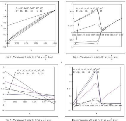
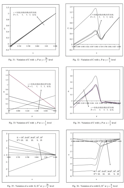
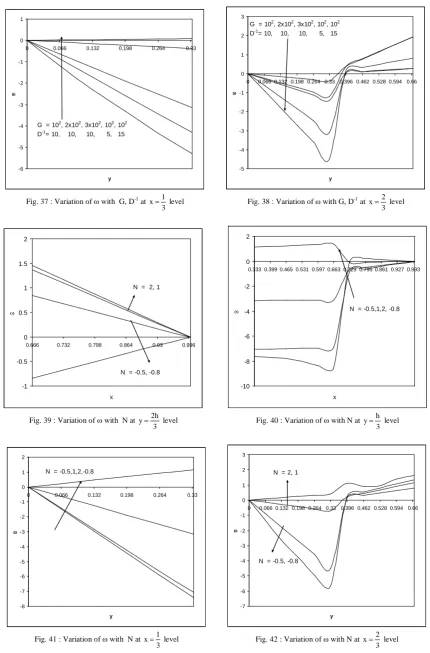
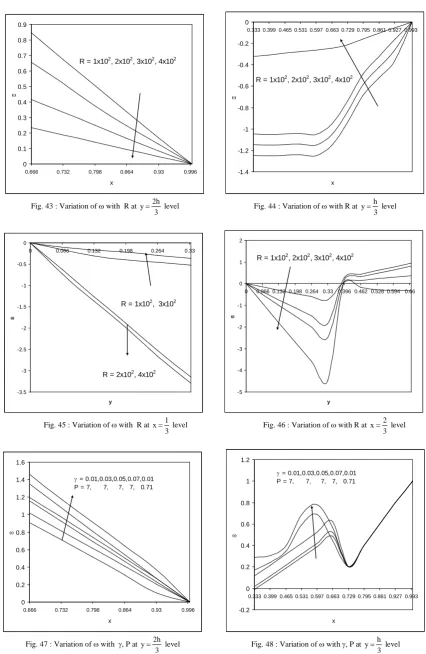
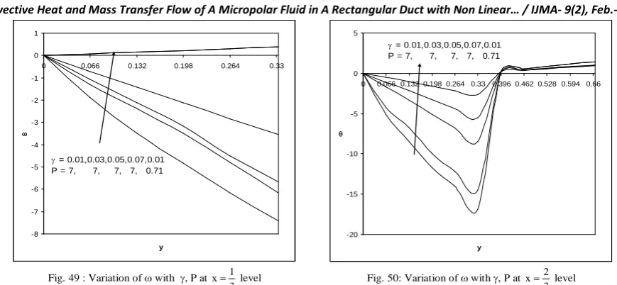
4. RESULTS AND DISCUSSION

In this analysis, we investigate the effect of non linear density temperature on convective heat and mass transfer flow of a micropolar fluid in a rectangular duct. The equations governing the flow of heat and mass transfer are non linear coupled equations. It is not possible to find closed form solutions; therefore we solve these equations by using Galerkin finite element analysis with three noded triangular elements. The temperature, concentration, angular velocity have

been analyzed for different values Grashof number (G), Darcy parameter (𝐷−𝐼), Buoyancy ratio (N), Micropolar

parameter (R), Schmidt number (Sc), Density ratio (γ), Prandtl number (P).

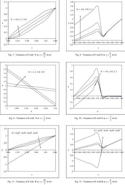
The temperature distribution (θ) is exhibited in figs (3-18) for different values G, 𝐷−𝐼, N, R, γ and P at horizontal levels Y= h/3 and Y=2h/3 and vertical levels X=1/3 and 2/3. We follow the convention that the non - dimensional

temperature (θ) is Positive or negative according as the actual temperature (T) is greater or lesser than Tc, the temperature on cold wall. From figs (3-6) we find that an increase in the Grashof number (G) enhances the actual temperature at Y=2h/3 and x=1/3 levels while at the levels y=h/3 and x=2/3, the actual temperature enhances with increase in G ≤ 3X 102 and reduces with higher G ≥ 5X 102 .The variation of θ with D-1 shows that lesser the

permeability of the porous medium (D-1≤10) larger the actual temperature at Y=h/3,2h/3 and X= 2/3 levels and smaller

at X=1/3 level, for further lowering of the permeability larger the actual temperature at Y=2h/3 and x=1/3 levels and

smaller at Y=h/3 and x=2/3 levels. The variation of θ with buoyancy ratio (N) is exhibited in figs (7-10) for different levels. It is found that when the molecular buoyancy force dominates over the thermal buoyancy force the actual temperature reduces at all the levels when the buoyancy forces are in the same direction and for the forces acting in opposite direction, the actual temperature enhances at both horizontal levels and vertical level X=2/3 and while at the vertical level X=1/3, it reduces in the flow of region. Figs (11-14) represent the variation of θ with Micropolar parameter (R). It is found that an increase in R ≤ 200, reduces the actual temperature and enhances with higher R ≥ 300 at Y=h/3, Y=2h/3 and X=2/3 levels. At X=1/3 level, the actual temperature enhances with lower and higher values of R and reduces with intermediate value of R = 200. Figs (15-18) represent of θ with density ratio (γ) shows that an

increase in γ≤0.03 reduces the actual temperature and enhances at higher values of γ≥0.05 at y=h/3, 2h/3 and x=1/3 levels. At x=2/3 level, the actual temperature reduces in the horizontal strip except in the region (0≤y≤ 0.132) enhances

with higher γ=0.05 and again reduces for still higher at γ=0.07 (Figs.15-18). The variation of θ with prandtl number (Pr) shows that lesser the thermal conductivity smaller the actual temperature at y=2h/3 and x=1/3 levels and larger at y=h/3 at x=2/3levels.

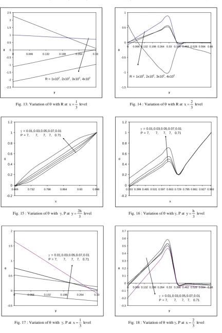
The non-dimensional concentration distribution (C) is shown in figs (19-34) for different parametric values at different horizontal and vertical levels. We follow the actual concentration enhances with G ≤ 3×102 and reduces with G ≥ 5×102 at both horizontal levels. At x=1/3 level it enhances with G. At higher vertical level x=2/3 level, the actual concentration enhances in the horizontal strip (0.132,0.066) and reduces in the region (0,0.66) with increase in G and the reversed effect is noticed in the behavior of the actual concentration in the above horizontal strip with higher G=5. Figs (23-26) represent the concentration with buoyancy ratio (N). It is found that when the molecular buoyancy force dominates over the thermal buoyancy force the actual concentration reduces at y=h/3 and x=1/3 levels irrespective of the directions of buoyancy forces. At y=2h/3 and x=2/3 levels, the actual concentration reduces with increase in N > 0

and enhances with increase │N │ (=0). Figs 27-30 represent the variation of C with micro polar parameter (R). It is

found that the actual concentration reduces with increase in R ≤ 100 and enhances with higher R ≥ 200. At y=h/3, 2h/3