Volume 2 (2006)
Proceedings of the
Workshop on Petri Nets and Graph Transformation
(PNGT 2006)
A basic tool for the modeling of
Marked-Controlled Reconfigurable Petri Nets
Marisa Llorens and Javier Oliver
13 pages
A basic tool for the modeling of
Marked-Controlled Reconfigurable Petri Nets
Marisa Llorens1and Javier Oliver2
1[email protected], 2[email protected]
Departamento de Sistemas Inform´aticos y Computaci´on (DSIC) Universidad Polit´ecnica de Valencia (UPV), Valencia, Spain
Abstract: In previous studies, we have introduced marked-controlled net rewrit-ing systems and a subclass of these called marked-controlled reconfigurable Petri nets. In a marked-controlled net rewriting system, a system configuration is de-scribed as a Petri net, and a change in configuration is dede-scribed as a graph rewriting rule. A marked-controlled reconfigurable Petri net is a marked-controlled net rewrit-ing system where a change in configuration amounts to a modification in the flow relations of the places in the domain of the involved rule in accordance with this rule, independently of the context in which this rewriting applies. In both mod-els, the enabling of a rule not only depends on the net topology, but also depends on the net marking according to control places. Even though the expressiveness of Petri nets and controlled reconfigurable Petri nets is the same, with marked-controlled reconfigurable Petri nets, we can easily and directly model concurrent and distributed systems that change their structure dynamically. In this article, we present MCReNet, a tool for the modeling and verification of marked-controlled reconfigurable Petri nets.
Keywords:structural dynamic changes, modeling, verification, tools.
1 Introduction
In [BLO03, Llo03, LO04b], we introduced the model of net rewriting systems (NRS) and a
subclass of this model,reconfigurable Petri nets(RN), to analyze, simulate and verify concurrent and distributed systems that are subject to structural dynamic changes. Both models arise from two different lines of research that were conducted in the field of the Petri net formalism [Mur89,
Pet81]. The goal of these lines of research is to enhance the expressiveness of the basic model
In [LO04a], we introduced marked-controlled net rewriting systems(MCNRS) and marked-controlled reconfigurable Petri nets(MCRN) as an extension of net rewriting systems and recon-figurable Petri nets, respectively, where the enabling of a rewriting rule not only depends on the net topology, but also depends on the net marking according to some net places namedcontrol places. In MCNRS, a system configuration is described as a Petri net, and a change in configura-tion is described as a graph rewriting rule, which consists of replacing part of the system (the part that matches the left-hand side of the rewriting rule) with another one (given by the right-hand side of the rewriting rule). A MCRN is a MCNRS where a change in configuration is limited to the modification of the flow relations of the places in the domain of the rewriting rule involved; i.e., the set of places and transitions is left unchanged by rewriting rules.
We are interested in developing a software tool to analyze the structure and dynamic behavior of systems that are modeled using our nets in order to evaluate them and suggest improvements or changes. The goal of our MCReNet tool is to study real systems that are modeled by MCRN. Our work is closely related to the topic of net transformation systems. There are some works in this area that perform the modification of the net topology and the modification of the system current marking. These works cover the modification of Petri nets in a categorical instead of a set theoretical way [EGP00]. In [LO04a] a detailed related work with respect to our models is presented. In [LKL05], a hybrid process mining approach to dynamic business process is pro-posed. The approach is based on reconfigurable Petri nets. This paper gives a method of mining dynamic changes in different instances; finally, a Reconfigurable Workflow Net is generated. In
[Akr05], a framework for managing changes in service oriented enterprises (SOEs) is presented.
The author presents a taxonomy of changes using a combination of several types of Petri nets to model the triggering changes and ensuing reactive changes. These changes are modeled by reconfigurable Petri nets.
The remainder of the paper is organized as follows. Section 2 recalls marked-controlled re-configurable Petri nets with an illustrative example and presents two algorithms: the first one (previously defined in a formal way in [LO04a]) translates marked-controlled reconfigurable Petri nets into Petri nets and the second one, in the opposite direction, obtains the current state of the marked-controlled reconfigurable Petri net from its equivalent Petri net. In Section 3, we describe the MCReNet tool in detail. Finally, Section 4 presents our conclusions.
2 Marked-Controlled Reconfigurable Petri nets
This section recalls the model of marked-controlled reconfigurable Petri nets introduced in
[LO04a].
2.1 Syntax and semantics
Definition 1 (Marked-Controlled Reconfigurable Petri net) Amarked-controlled reconfig-urable Petri net (MCRN)[LO04a] is a structure N= (P,T,R,γ0), where P={p1, . . . ,pn}is a non-empty and finite set of places; T ={t1, . . . ,tm}is a non-empty and finite set of transitions
Arewriting rule r∈Ris a structurer= (D,•r,r•,C,M), where:
• D⊆Pis thedomainofr;
• •r :(D×T)∪(T×D)→N and r•:(D×T)∪(T×D)→N are the preconditions and
postconditionsof r, (i.e. they are the flow relations of the domain places before and after the change in configuration due to ruler);
• Cis a subset of places ofD,C⊆D, calledcontrol places, and
• Mis the required minimum marking of places ofCso that the rule can be enabled.
Aconfigurationof a MCRN is a Petri netΓ= (P,T,F).
Astateγ of a MCRN is a marked Petri netγ= (Γ,M). The stateγ0is called theinitial state
of the MCRN.
Theeventsof a MCRN are the transitions and the rewriting rules:E=T∪R.
We represent a rewriting rule using formal sums notation as r=∑p∈Dp(∑t∈T •r(p,t)·t−∑
t∈T •r(t,p)·t)B∑p∈Dp(∑t∈Tr•(p,t)·t−∑t∈Tr•(t,p)·t) Definition 2 (Configuration Graph of a MCRN) Theconfiguration graph G(N)of a MCRN N= (P,T,R,γ0)is the labeled directed graph whose nodes are the configurations, such that there is an arc from configurationΓto configurationΓ0labeled with ruler= (D, •r, r•,C, M)∈R,
which we denoteΓ[riΓ0, if and only if the following holds: ∀p∈C: M(p)≥M(p)
∀p∈D:
F(p,t) = •r(p,t)andF(t,p) = •r(t,p)
F0(p,t) =r•(p,t)andF0(t,p) =r•(t,p)
∀p∈/D: F(p,t) =F0(p,t)andF(t,p) =F0(t,p)
Notice that we require the control places to be marked with at least markingM. The transition
relation must contain arcs of the exact multiplicity appearing in the left-hand side of the rewriting rule, and we do not allow rewriting if arcs of a greater multiplicity are present.
The dynamic evolution of a MCRN is then given by its state graph.
Definition 3 (State Graph of a MCRN) Thestate graphof a MCRNN= (P,T,R,γ0)is the labeled directed graph whose nodes are states ofNand whose arcs (labeled with events) are of two kinds:
1. firing of a transition:arc from state(Γ,M)to(Γ,M0)that is labeled with transitiont when t can fire in the netΓat markingMand leads toM0, and
2. change in configuration: arc from state(Γ,M) to state (Γ0,M) that is labeled with rule r∈RifΓ[riΓ0is a transition of the configuration graph ofN.
In other words, the set of labeled arcs of the state graph ofNis given by
2.2 Example
The following example shows a system modeled by a MCRN, and a change in configuration that depends on both the net topology and the net marking. We have chosen an example that is related to manufacturing processes since, in these types of problems, changes in the structure are very frequent and they usually depend on the state of the manufacturing processes.
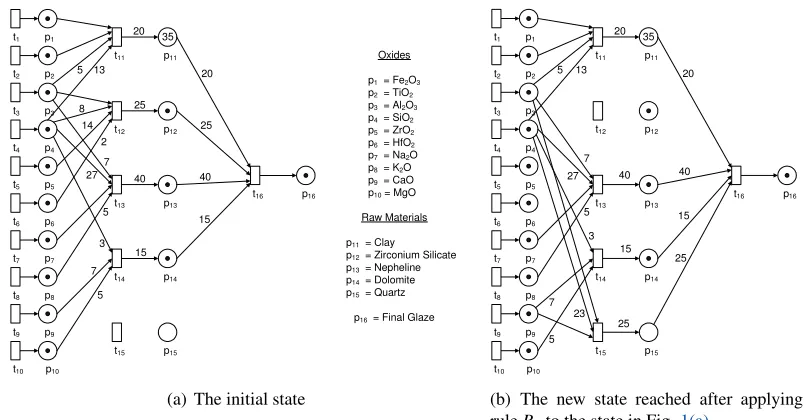
Example1(Glaze Manufacture) In the manufacturing process of a glaze, different glazes are made by using different raw materials that, after firing, have certain characteristics.
t1 t2 t3 t4 t11 t5 t6 t7 p1 p2 p3 p4 p5 p6 p7
t8 p8
t9 p9
t10 p10
p11
t12 p12
t13 p13
t14 p14
t15 p15
t16 p16
Oxides p1 = Fe2O3 p2 = TiO2 p3 = Al2O3 p4 = SiO2 p5 = ZrO2 p6 = HfO2 p7 = Na2O p8 = K2O p9 = CaO p10 = MgO Raw Materials p11 = Clay p12 = Zirconium Silicate p13 = Nepheline p14 = Dolomite p15 = Quartz
p16 = Final Glaze 20 20 25 25 40 40 15 15 5 13 8 14 2 27 5 7 3 7 5 35
(a) The initial state
t1 t2 t3 t4 t11 t5 t6 t7 p1 p2 p3 p4 p5 p6 p7
t8 p8
t9 p9
t10 p10
p11
t12 p12
t13 p13
t14 p14
t15 p15
t16 p16
25 25 40 40 15 15 20 20 5 13 27 5 7 3 7 5 23 35
(b) The new state reached after applying
ruleR1to the state in Fig.1(a)
Figure 1: Two states of the MCRN of Example1
p3 p4 p5 p6 p9
t12 p12
t15 p15 t16 p3 p4 p5 p6 p9
t12 p12
t15 p15 t16 R1 25 25 25 25 8 14 2 23
(a) RuleR1
t11 p1 p2 p3 p4 p9 p10 p11
t14 p14 t16 t11 p1 p2 p3 p4 p9 p10 p11
t14 p14 t16 R2 15 15 20 20 35 35 3 7 5 10 22 5 13 2
(b) RuleR2
Figure 2: Rewriting rulesR1andR2of the MCRN of Example1
opaque glaze turns into a semi-opaque glaze with a high LDC. If we remove all of the dolomite and increase the clay, we obtain a glaze that water marks and that is disk-glazed. Changing the composition of the glaze in our model means changing the net topology. To make these changes possible, we define two rewriting rules using the formal sums notation previously introduced. We show them (R1andR2) graphically in Fig.2(a)and Fig.2(b), respectively. The subset of control
placesCis empty for rule R1, whereas, for ruleR2, this subset isC={p11}and M(p11) =35 (i.e., to remove all of the dolomite and increase the clay, at least 35%clay is needed in place
p11). Therefore, the MCRN consists of 16 places, 16 transitions, and 2 rewriting rules.
R1: p3(-t12)+p4(-8t12)+p5(-14t12)+p6(-2t12)+p9(/0)+p12(25t12-25t16)+p15(/0)
B
p3(-t15)+p4(-23t15)+p5(/0)+p6(/0)+p9(-t15)+p12(/0)+p15(25t15-25t16)
R2: p1(-t11)+p2(-t11)+p3(-5t11)+p4(-13t11-3t14)+p9(-7t14)+p10(-5t14)+p11(20t11-20t16)+p14(15t14-15t16)
B
p1(-t11)+p2(-2t11)+p3(-10t11)+p4(-22t11)+p9(/0)+p10(/0)+p11(35t11-35t16)+p14(/0)
Figure1(b)shows the state that is reached when ruleR1(in Fig. 2(a)) is applied to the initial
state represented in Fig.1(a). In this new state, all the zirconium silicate has been substituted by quartz.
There are only four possible configurations. The initial configurationΓ0and the configuration Γ1are the configurations of the states represented in Fig.1(a)and Fig.1(b), respectively.
2.3 Relationship between Petri nets and MCRNs
In [LO04a], we prove that MCRNs are equivalent to Petri nets, but they provide somewhat more
compact representations of concurrent and distributed systems whose structure evolves at run-time. The substantial increase in the number of transitions with respect to the MCRN implies that the size of the Petri net grows considerably. This can be observed in Fig. 4that shows the Petri net (20 places, 72 transitions) equivalent to the MCRN of Example1. Watching this figure, we can imagine how big the entire Petri net is and how we can best model the system with a MCRN.
The Petri netN∼ = (P∼,T∼,F∼,M∼)equivalent to a MCRNN= (P,T,R,γ0)is obtained following Algorithm 1, that is completely defined in a formal way in [LO04a]. The set of places ∼P is P∪ {q0, . . . ,qk}, where P is the set of places of the original MCRN and each placeqi is one
specific place attached to each possible configurationΓi∈G(N). The marking
∼
Mfor places of the subsetPis the marking that they have in the initial stateγ0of the MCRNNand for the added
places {q0, . . . ,qk}is 0 except for placeq0whose marking is 1. This marking shows that Γ0 is
the current configuration.
Now, we have developed an algorithm that acts in the other direction. That is, it is possible to extract the stateγi= (Γi,Mi)of a MCRN from the corresponding marked Petri net
∼
N= (P∼,T∼,F∼,
∼
M), at a given moment, following Algorithm 2. This algorithm starts from a marked Petri net,
Algorithm 1Petri Net equivalent to a Marked-Controlled Reconfigurable Petri net
1: We start from the initial configurationΓ0. ForΓ0, we obtain all the possible configurations
due to the firings of all enabled rewriting rules, that is, we obtain all the nodes of the first level of the configuration graphG(N). If we imagine places and transitions of a configuration as if they were located in two different parallel planes, i.e., a plane with the set of places and a plane with the set of transitions connected by the flow relations of the represented configuration, we will have only one plane of places, and as many planes of transitions as there are different configurations.
2: For each plane of transitions we add a placeqi, connected by an input arc and an output arc
with all transitions of the plane.
3: We also add a transitionr0ibetween placeq0of the initial configuration and each planeqiof
each reachable configuration fromq0; this represents the change in configuration due to rule r,Γ0[riΓi.
4: If there are control places involved in the change in configurationΓ0[riΓi, we connect
tran-sitionr0iwith each control place of rule r(in the plane of places) using an input arc and an
output arc whose weight is the required minimum marking of the control place for the rule to be enabled.
5: We repeat this process for each configuration that is distinct from the initial configuration, that is, for each plane of transitions obtained from the initial plane.
starting point, it is not very difficult to distinguish the subnet that represents the current state of the initial MCRN (the input of Algorithm1).
Theorem 1 It is possible to extract the stateγi= (Γi,Mi)of a MCRN from the corresponding
marked Petri netN∼= (P∼,T∼,F∼,M∼), at a given moment.
Proof. The corresponding marked Petri netN∼ has been obtained from Algorithm1. It is straight-forward to extract the stateγi= (Γi,Mi)of a MCRN following Algorithm2.
3 The MCReNet Software Tool
To study real systems that are modeled by MCRN, it would be useful to have a software tool to analyze the structure and dynamic behavior of the modeled system in order to evaluate it and suggest improvements or changes. The MCRN model is equivalent to the Petri net model and, therefore, the decidable properties of Petri nets are still decidable for our model. It is possible to obtain an automatic verification tool for MCRN. Our objective is to develop a tool to design and verify systems modeled by MCRN. This tool has a graphical editor, a simulator and an analyzer for several common properties.
Algorithm 2 State of a Marked-Controlled Reconfigurable Petri Net from the corresponding Petri Net
1: We start from the marked Petri net N∼ = (P∼, T∼, F∼, M∼) where ∼P is the set of places ∼P= P∪ {q0, . . . ,qk},
∼
T is the set of transitionsT∼= ({q0, . . . ,qk} ×T) ∪
∼
R,F∼is the flow relation andM∼ is the marking of the net.
2: At markingM∼, ∑k
j=0 ∼
M(qj) =1, that is, only one placeqi of the subset of places{q0, . . . ,qk}
is marked with one token. From the subset of transitions {q0, . . . ,qk} ×T ∈
∼
T only the transitions in{qi} ×T are enabled.
3: The current stateγi= (Γi,Mi)of MCRN is composed by:
• the current configurationΓi = (Pi,Ti,Fi)where the set of places is Pi=P, the set of
transitions isTi={qi} ×T, and the flow relationFiis given by
∀p∈Pi,∀t∈Ti:
(
Fi(p,t) =
∼
F(p,(qi,t))
Fi(t,p) =
∼
F((qi,t),p)
• the current markingMiis Mi(p) =
∼
Mi(p) ∀p∈P
• both the initial state and the rewriting rules of a MCRN are Petri nets;
• a MCRN is formally equivalent to a Petri net;
• an algorithm that obtains an equivalent Petri net from a MCRN is available (Algorithm1).
The idea is to use an already existing graphical editor of Petri nets to draw the initial MCRN, i.e., a Petri net. Our tool will use this net:
1. To make a syntactical analysis of the files generated by the editor and to store the relevant information in the suitable data structures.
2. To implement the algorithm to translate a MCRN into an equivalent Petri net.
3. To create a file (from the resulting Petri net) that can be viewed from the editor.
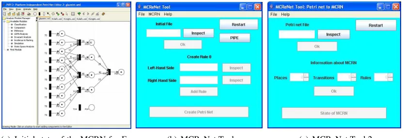
We have chosen PIPE (Platform Independent Petri net Editor) [Webc, BCC+04,Akh05], a
free software for non business use that allows the design, analysis, and simulation of Petri nets. This editor allows us to create, save and load Petri nets according to the last standard XML for Petri nets, PNML (Petri Net Markup Language[Webd]).
(a) Initial state of the MCRN for
Ex-ample1in PIPE
(b) MCReNet Tool (c) MCReNet Tool 2
Figure 3: Main screens of PIPE and MCReNet Tool
for Example1. The background windows contain the left and right-hand sides of the rewriting rules.
Various XML files are obtained (one for the initial state, and two for each one of the rewriting rules). These XML files have a well-defined structure where the division between places, transi-tions, and arcs is clearly visible. Any file of this type has a headline that shows what language is used, here PNML [Webd]. Next, the name and the type of the represented net appear.
<?xml version="1.0" encoding="iso-8859-1" ?> <pnml> <net id="Net-One" type="P/T net">
For every place appears an identifier, the graphic coordinates, a label, and the initial marking. For every transition appears an identifier, the graphic coordinates, a label, the orientation, a rate, and if it is timed or not.
<place id="P0"> <transition id="T0"> <graphics> <graphics>
<position x="90.0" y="60.0" /> <position x="30.0" y="60.0" /> </graphics> </graphics>
<name> <name>
<value>P0</value> <value>T0</value> <graphics /> <graphics /> </name> </name>
<initialMarking> <orientation> <value>1</value> <value>0</value> <graphics> </orientation>
<offset x="0.0" y="0.0" /> <rate>
</graphics> <value>1.0</value> </initialMarking> </rate>
</place> <timed>
<value>false</value> </timed>
</transition>
<arc id="T0 to P0" source="T0" target="P0"> <arc id="P0 to T0" source="P0" target="T0"> <graphics /> <graphics />
<inscription> <inscription> <value>2</value> <value>5</value> <graphics /> <graphics /> </inscription> </inscription>
<arcpath id="000" x="45" y="71" <arcpath id="000" x="115" y="70" curvePoint="false" /> curvePoint="false" />
<arcpath id="001" x="86" y="71" <arcpath id="001" x="156" y="70" curvePoint="false" /> curvePoint="false" />
</arc> </arc>
After this information, the headline labels are closed. </net>
</pnml>
Figure3(b)shows the initial screen of the MCReNet Tool. User introduces the XML files that represent the initial state and the left-hand and right-hand side of all rules from this screen.
A syntactical analysis of these files is made in order to extract the information from them. The name and its marking are obtained for each place. The name is obtained for each transition. The weight and the places and transitions that the arc connects are obtained for each arc (the incidence matrix of the net [Mur89]). A consistency check is made, that is, it is checked whether the initial net together with pairs of nets representing rules create a MCRN (whether they differ only in the flow relation). Since both the left-hand side and the right-hand side of the rules are Petri nets with identical places and identical transitions, besides knowing its names, we are interested in knowing the flow relation between them in each part of the rule (the incidence matrix of the left-hand side and the incidence matrix of the right-hand side of the rewriting rule).
The process of translation begins when user presses theCreate Petri netbutton. The translator that obtains the Petri net that is equivalent to the initial MCRN is implemented in Java [Weba] following Algorithm 1. The first step of this algorithm is to obtain the configuration graph G(N)of the initial MCRN. We obtain a procedure that (from the initial state and the rewriting rules) checks which rules are enabled and it obtains the resulting configurations of the firings of these rules. The process is repeated for each one of the obtained configurations, as long as new configurations are obtained and until no more rules are firable. All the possible configurations of the MCRN must be stored indicating which configurations are immediately reachable from a given configuration, due to the firing of which rules.
OnceG(N)is obtained, the tool is ready to translate this net into its equivalent Petri net. Ac-cording to Algorithm 1, the translation process consists in adding new places, new transitions, and their corresponding flow relations to the places and transitions of the initial configuration. Since the number of places and transitions of the equivalent Petri net is known [LO04a], the dimensions of the incidence matrices can be known. The previous and posterior incidence matri-ces are filled according to the flow relations of the configurations ofG(N). A file with the same format as the PIPE files is obtained from the resulting Petri net. Therefore, this Petri net can be displayed on the PIPE editor (see Fig.4).
After obtaining the equivalent Petri net, the process of analysis and simulation can begin. The PIPE editor itself offers the possibility of doing simulation and analysis of properties. Figures
Figure 4: Petri net equivalent to the MCRN of Example1in PIPE
transitions, (b) the invariant analysis and (c) the incidence and marking matrices and the enabled transitions set.
(a) The classification results (b) The invariant analysis (c) The incidence matrices
Figure 5: Some analyses of the Petri net of Fig.4
4 Conclusions and further work
We have developed a tool to analyze, simulate, and verify systems that are modeled with MCRN. On the basis of the equivalence between Petri nets and MCRN, we have initially opted to develop a tool that exploits the capabilities of the Petri net tools that are currently available. The main goal of our tool is the implementation of a translation algorithm of a MCRN into an equivalent Petri net (Algorithm1). We have chosen PIPE as the graphical editor, simulator and analyzer. MCReNet integrates PIPE with the translator. Therefore, user can draw the initial state and rewriting rules of the MCRN, which is then translated into its equivalent Petri net. In addition, a simulation and an analysis of properties of this net can be performed. All these processes are integrated in the MCReNet tool. The other goal of our tool is the implementation of Algorithm
2to obtain the current state of a MCRN from its equivalent Petri net at a given moment.
As further work, we will develop a tool that is completely autonomous. Our new tool will be able to directly carry out the editing, simulation and analysis of net properties on MCRN. We are currently working on the theoretical aspects of the analysis methods for Petri nets in order to ap-ply them directly to MCRN. Also we are studying the relationships between our approaches and other existing proposals using rewriting techniques for providing a reconfiguration mechanism for Petri nets (like, e.g., open Petri nets [BCE+06] and high-level replacement systems applied
to Petri nets [PER95,HEM05]).
Acknowledgements: This work has been partially supported by the EU (FEDER) and the Spanish MEC under grant TIN2005-09207-C03-02 and by the ICT for EU-India Cross-Cultural Dissemination Project ALA/95/23/2003/077-054.
Bibliography
[Akh05] N. Akharware. PIPE2: Platform Independent Petri Net Editor. Msc. project report, Department of Computing, Imperial College, London, 2005.
[Akr05] M. S. Akram. Managing Changes to Service Oriented Enterprises. Master’s thesis, Virginia Polytechnic Institute and State University, USA, 2005.
[Bal00] P. Baldan. Modelling Concurrent Computations: From Contextual Petri Nets to Graph Grammars. Phd thesis, Computer Science Department, University of Pisa, Italy, 2000.
[BCC+04] T. Barnwell, M. Camacho, M. Cook, M. Gready, P. Kyme, M. Tsouchlaris. PIPE.
Platform Independent Petri-net Editor. Final report, Petri Net Analyser - Group 4. Department of Computing, Imperial College, London, 2004.
[BCE+06] P. Baldan, A. Corradini, H. Ehrig, R. Heckel, B. Knig. Bisimilarity and
[BLO03] E. Badouel, M. Llorens, J. Oliver. Modelling Concurrent Systems: Reconfigurable Nets. In Arabnia and Mun (eds.), Int. Conf. on Parallel and Distributed Process-ing Techniques and Applications (PDPTA’03). Volume IV, pp. 1568–1574. CSREA Press, Las Vegas, Nevada (USA), June 23-26 2003.
[Cor95] A. Corradini. Concurrent Computing: From Petri Nets to Graph Grammars. Elec-tronic Notes in Theoretical Computer Science2, 1995. Invited talk at theJoint COM-PUGRAPH/SEMAGRAPH Workshop on Graph Rewriting and Computation.
http://www.elsevier.nl/locate/entcs/volume2.html
[EGP00] H. Ehrig, M. Gajewsky, F. Parisi-Presicce. High-Level Replacement Systems Ap-plied to Algebraic Specifications and Petri Nets. InHandbook of Graph Grammars and Computing by Graph Transformation, Vol. III: Concurrency, Parallelism and Distribution. Pp. 341–400. World Scientific, 2000.
[HEM05] K. Hoffmann, H. Ehrig, T. Mossakowski. High-Level Nets with Nets and Rules as Tokens. In Ciardo and Darondeau (eds.), Proc. 26th Int. Conf. on Applications and Theory of Petri Nets (ICATPN’05). Lecture Notes in Computer Science 3536, pp. 268–288. Springer, Miami, USA, June 20-25 2005.
[LKL05] N. Li, J. Kang, W. Lv. A Hybrid Approach for Dynamic Business Process Min-ing Based on Reconfigurable Nets and Event Types. InProc. IEEE Int. Conf. on e-Businees Engineering (ICEBE’05). Pp. 289–294. IEEE Computer Society, Beijing, Peoples Rep. China, 2005.
[Llo03] M. Llorens. Redes Reconfigurables. Modelizaci ´on y Verificaci´on. Phd thesis (in spanish), Departamento de Sistemas Inform´aticos y Computaci´on, Universidad Polit´ecnica de Valencia, Spain, 2003.
[LO04a] M. Llorens, J. Oliver. Introducing Structural Dynamic Changes in Petri Nets: Marked-Controlled Reconfigurable Nets. In Proc. Int. Conf. on Automated Tech-nology for Verification and Analysis (ATVA’04). Lecture Notes in Computer Sci-ence 3299, pp. 310–323. Springer Verlag, Taipei, Taiwan, 2004.
[LO04b] M. Llorens, J. Oliver. Structural and Dynamic Changes in Concurrent Systems: Reconfigurable Petri Nets. IEEE Transactions on Computers 53(9):1147–1158, September 2004.
[Mur89] T. Murata. Petri Nets: Properties, Analysis and Applications. InProc. of the IEEE. Volume 77(4), pp. 541–580. April 1989.
[PER95] J. Padberg, H. Ehrig, L. Ribeiro. Algebraic High-Level Net Transformation Systems. Mathematical Structures in Computer Science5(2):217–256, 1995.
[Sch94] H. Schneider. Graph Grammars as a Tool to Define the Behavior of Processes Sys-tems: From Petri Nets to Linda. InFifth International Conference on Graph Gram-mars and their Application to Computer Science. Pp. 7–12. Williamsburg, USA, 1994.
[Val78] R. Valk. Self-Modifying Nets, a Natural Extension of Petri Nets. In Ausiello and Bhm (eds.), Proc. of the 5th Int. Coll. Automata, Languages and Programming (ICALP’78). Lecture Notes In Computer Science 62, pp. 464–476. Springer-Verlag, Udine, Italy, 1978.
[Val81] R. Valk. Generalizations of Petri Nets. In Gruska and Chytil (eds.), Proc. of 10th. Symposium on Mathematical Foundations of Computer Science (MFCS’81). Lec-ture Notes in Computer Science 118, pp. 140–155. Springer-Verlag, Strbske Pleso, Czechoslovakia, 1981.
[Weba] Sun’s Home for Java:http://java.sun.com/.
[Webb] The Home Page of Petri Net Tools on the Web:http://www.informatik.uni-hamburg.
de/TGI/PetriNets/tools/.
[Webc] The Home Page of PIPE:http://pipe2.sourceforge.net/.