Internet Nameserver IPv4 and IPv6 Address Relationships
Arthur Berger
MIT CSAIL / Akamai
awberger@csail.mit.edu
Nicholas Weaver
ICSI / UCSDnweaver@icsi.berkeley.edu
Robert Beverly
Naval Postgraduate Schoolrbeverly@nps.edu
Larry Campbell
Akamai
lcampbel@akamai.com
ABSTRACT
The modern Domain Name System (DNS) provides not only resolution, but also enables intelligent client routing, e.g. for Content Distribution Networks (CDNs). The adoption of IPv6 presents CDNs the opportunity to utilize different paths when optimizing traffic, and the challenge of appro-priately mapping IPv6 DNS queries. This work seeks to dis-cover the associations between Internet DNS client resolver IPv6 address(es) and IPv4 address(es). We design and im-plement two new techniques, one passive and one active, to gather resolver pairings. The passive technique, deployed in Akamai’s production DNS infrastructure, opportunistically discovered 674k (IPv4, IPv6) associated address pairs within a six-month period. We find that 34% of addresses are one-to-one, i.e. appear in no other pair, a fraction that increases to ≈ 50% when aggregating IPv6 addresses into /64 pre-fixes. The one-to-one associations are suggestive, but not a sufficient condition, of dual-stack DNS recursive resolvers. We further substantiate our inferences via PTR records and software versions, and manual verification of sample pairings by three major Network Operators. Complex associations, where e.g. distributed DNS resolution leads to inferred ad-dress groupings that span continents and many autonomous systems exist, a subset of which we explore in more depth using the active probing technique. Among potential uses, Akamai is currently utilizing screened output from the pas-sive technique, in conjunction with prior knowledge of IPv4, to inform IPv6 geolocation within its CDN.
Categories and Subject Descriptors
C.2.3 [Computer Communication Networks]: Network Operations—network monitoring
General Terms
Measurement, Experimentation
(c) 2013 Association for Computing Machinery. ACM acknowledges that this contribution was authored or co-authored by an employee, contractor or affiliate of the United States government. As such, the United States Gov-ernment retains a nonexclusive, royalty-free right to publish or reproduce this article, or to allow others to do so, for Government purposes only.
IMC’13,October 23–25, 2013, Barcelona, Spain. Copyright 2013 ACM 978-1-4503-1953-9/13/10 ...$15.00. http://dx.doi.org/10.1145/2504730.2504745.
Keywords
DNS; Nameservers; Resolvers; IPv6
1. INTRODUCTION
After languishing for decades, IPv6 [13] is experiencing renewed interest [17], in large part due to economics and politics [10, 23]. However, IPv4 and IPv6 are expected to co-exist for the foreseeable future. Transition strategies, prac-tical constraints, and inertia imply that portions of the IPv6 infrastructure will depend on IPv4, where hosts and infras-tructure are “dual-stacked.”
Previous measurement research has explored IPv6 pene-tration of the broader client population, for instance via web instrumentation [11, 32, 27]. Several initiatives [18, 19] and anecdotal evidence [28] suggest that IPv6 infrastructure de-ployment is proceeding in advance of client adoption. For instance, many large residential networks [12] and content providers [1] fully support IPv6. An important component of any provider’s transition plans is enabling IPv6 on their Domain Name System (DNS) servers, including local recur-sive client resolvers.
Our motivation is interest in associating Internet DNS resolver IPv6 address(es) with IPv4 address(es). Opera-tionally, such association is especially important to Con-tent Distribution Networks (CDNs), where information of a client’s recursive resolver is used to perform intelligent client routing and load balancing. We are particularly interested the simple case of one-to-one associations as such pairs are candidates for being on the same machine, or even interface, and thus collocated, which can be used as an input to IPv6 geolocation.
Our work is concerned with developing techniques for as-sociating IPv4 and IPv6 DNS resolver addresses, and per-forming large-scale measurements to collect such associa-tions. While out of scope for the present paper, obtaining DNS resolver associations between the two protocols has sev-eral potential future applications:
1. Internet Evolution: As IPv6 deployment continues, the infrastructure supporting each protocol will evolve. The techniques herein can be used in the future for a longitudinal study of tracking the inter-relationship of IPv4 and IPv6 nameservers.
2. IPv6 Geolocation: There is potential to leverage prior knowledge of geolocation of IPv4 addresses [5] to inform IPv6 geolocation when the addresses are corre-lated. One-to-one DNS resolver associations are
con-sistent with, but not proof of, the corresponding IPv4 and IPv6 addresses being assigned to the same ma-chine, and thus being at the same physical location. Further screening of such pairs, discussed in§5.1, can pick out those that are more likely to be collocated. However, as with other inputs to geolocation, our asso-ciations are likely to be noisy and thus must be appro-priately weighted. Akamai Technologies is currently using screened output from the opportunistic passive technique,§2.1, in conjunction with prior knowledge of IPv4, as one of the inputs for IPv6 geolocation within its CDN.
3. Security: IPv4, IPv6 nameserver pairs that are likely on the same machine are of interest from a security viewpoint. Not only are many old IPv4 attacks fea-sible in IPv6 [7], IPv6 introduces new attack vectors [16]. An attack directed against the IPv6 address of a DNS server may also impact an organization’s corre-sponding IPv4 service.
Our hope is that our techniques and data from this re-search can be used as a first step toward future work on these important applications.
To this end, we develop two novel techniques for discov-ering associated IPv4 and IPv6 resolver addresses: i) a pas-sive, opportunistic technique that uses a two-level DNS hier-archy that encodes IPv4 addresses within IPv6 nameserver records; and ii) an active technique whereby we probe re-solvers to induce various lookup behaviors. Our techniques provide new methods to characterize a small, but critical, portion of the Internet infrastructure.
The passive technique has been implemented in the Aka-mai CDN, and for 674k (IPv4, IPv6) address pairs observed over a six month period, we find that 34% of the collected resolver addresses have a one-to-one association, i.e. appear in no other address pair. This percentage increases to al-most 50% when the IPv6’s are aggregated to /64 prefixes, (creating pairs of an IPv4 address with an IPv6 /64 pre-fix). We also discover complex, connected sets of address pairs that, at the extreme, span continents and hundreds of Autonomous Systems, where large cluster resolvers and public DNS providers play a major role. Additionally, we find evidence of abnormal use of 6to4 tunnels.
To help substantiate our results, we analyze the PTR records and software versions of the association inferences. For more precise validation of a subset of the associations, we employ our active measurement technique to perform a data collection over 13 hours to minimize temporal address assignment changes and corroborate the extant complexity discovered passively. Last, for samples sent to personal con-tacts at six major networks, three responded and manually confirmed that all of our inferred one-to-one associations that they checked were correct and indeed assigned to the same machine.
In total, this paper makes four primary contributions: 1. A new passive technique foropportunistically pairing
IPv4 and IPv6 addresses of DNS resolvers.
2. A novel approach for active, targeted, DNS resolver probing to discover associated address pairs.
3. Real-world deployment of the passive technique on a commercial CDN to gather a large cross section of In-ternet resolvers. src: IPv6, dst: 2001:428::IPv4 Pairs DNS Resolver IPv4 IPv6 NS=2001:428::IPv4 A? www.a.example.com (IPv4,IPv6) A? www.a.example.com SecondïLevel FirstïLevel Auth DNS Auth DNS
Figure 1: DNS Resolver IPv4/IPv6 Address Infer-ence: A multi-level authority returns second-level
nameserver AAAA records encoding a query’s IPv4
source in the lower-order bits. The second-level
nameserver associates IPv6 sources with the IPv4 encoded in the destination IPv6.
4. Analysis of observed DNS resolver address pairs that finds a significant proportion, 34%, have a one-to-one association (almost 50% when the IPv6’s are aggre-gated to /64 prefixes) and also finds complex, con-nected sets of address pairs.
The remainder of this paper is organized as follows. Sec-tion 2 details the two measurement techniques comprising our system as well as our deployment. We summarize the collected data in §3, present its analysis in§4, and discuss findings in§5. Finally, we conclude in§6 with a summary of implications and suggestions for future work.
2. METHODOLOGY
Our system includes two novel measurement techniques. First, we develop a passive, opportunistic method to dis-cover candidate IPv4 and IPv6 addresses of DNS resolvers. Second, we create a custom DNS server that permitsactive
measurement of DNS resolvers. In this section, we detail these techniques.
2.1 Opportunistic DNS Technique
Clients rely on local recursive resolvers to perform DNS resolution. We seek to ascertain the IPv4, IPv6 addresses of dual-stacked DNS resolvers by inducing them to reveal their addresses as part of their natural lookup process.
Our technique exploits: 1) a two-level authoritative DNS resolution, and 2) the ability to encode an IPv4 address in the lower order bits of an IPv6 address. For the purpose of exposition, assume we control, and deploy our technique on, the DNS authority ofexample.com.
Consider a recursive DNS resolver servicing a local client requesting resolution of www.a.example.com. As depicted in Figure 1, the resolver requests resolution (typically anA
record) for this host from the first-level authoritative name-server via an IPv4 DNS query. The first-level namename-server responds with the second-levelNS, and corresponding “addi-tional”AandAAAA, records [22]. Crucially, theAAAArecords of the second-levelNS, as returned by our first-level name-server, are formed dynamically. The first-level DNSencodes a query’s IPv4 source address in the lower-order bits of the response’s additionalAAAArecord.
For example, Figure 1 shows the first-level DNS respond-ing to a DNS resolver’s query with the authoritative NS
record of the second-level DNS, including an additionalAAAA
record for the second-level nameserver that includes the query-ing resolver’s IPv4 source address in the low-order bits. The
recursive DNS resolver may use either theAorAAAAaddress for the second-level resolution. When the latter is used, the second-level DNS can pair the IPv6 source address of the query it receives with the IPv4 address encoded in the IPv6 destination of the query. Note that the dynamically gener-atedAAAAnameserver record is valid as the second-level DNS accepts queries from an entire prefix; we use a /80 prefix.
Akamai Technologies has deployed this passive technique within its production infrastructure [26], making use of its pre-existing multi-level DNS hierarchy (whose primary pur-pose is to resolve names to CDN addresses that can best serve the client), and has activated it for a selection of do-mains. Akamai has used the resulting data collection during the revision of its request-routing software to support IPv6, and continues to use it as one of the inputs into Akamai’s geolocation product [5] where the extensive prior knowledge of IPv4 can be used to aid in the location of IPv6 when the IPv4 and IPv6 addresses are inferred to be correlated.
As a practical issue, the first-level authoritative DNS in Figure 1 does not know whether the client’s nameserver is IPv6 capable, as the incoming DNS query arrives over IPv4. Thus, in Akamai’s implementation, of eightNSrecords returned, only one or two of the associated glue records are AAAA. Also, even when the client’s nameserver is dual stacked, it may not select theAAAA; selection order typically depends on historical load and performance characteristics. Note that this technique is opportunistic: a client resolver must first contact our authoritative DNS for resolution of an object within our portion of the DNS namespace. No additional packets are sent when one deploys the technique for domain names that are being used anyway. Because the technique is passive, where the collection of address pairs is simply a by-product of the client’s resolver requesting a domain under our authority, there are no restrictions on the population of resolvers we can measure. In particular, we are not limited to open resolvers as the entity collecting the data is not initiating the DNS query.
Also note that the passive technique only checks whether the client’s resolver can send IPv6, but does not check whether it can receive IPv6. If it can not receive responses over IPv6, the query will timeout, and the resolver can fallback to retry using an IPv4 glue record. In such a scenario, we still record an (IPv4, IPv6) pair. This ambiguity does not occur with the active technique of§2.2.
The passive technique can be implemented on any au-thoritative nameservers under common control along a DNS namespace hierarchy. It can be implemented even on a sin-gle machine, with multiple addresses, where the IPv4 glue address for the NS record forexample.comis distinct from the IPv4 and IPv6 glue addresses for the NS record that causes the lookup to the second level. However, our deploy-ment using separate first and second-level authorities is most compatible with the existing Akamai infrastructure, where deployment on Akamai affords us a rich and diverse dataset.
2.1.1 Advantageous Complications
Figure 1 illustrates the simple case where the DNS queries come from a single, dual-stacked machine. However, the reality of Internet DNS resolution can be much more com-plex. Recall that the (IPv4, IPv6) addresses that are logged are addresses seen by the authoritative nameservers. They need not be associated with the same machine. It is well-known that DNS servers and resolvers experience significant
load, and that many approaches exist for balancing DNS query load [25, 3, 15, 4]. A relatively common case, espe-cially among large providers, is that a provider maintains a set of servers at a location that share the load, and also may share a cache or may distribute obtained resolutions. Further, DNS resolver implementations may perform record pre-fetching [4] in an effort to improve performance.
In Akamai’s implementation, theNSrecords returned by the first-level authoritative DNS have a TTL of 12 hours. Thus, if there is shared cache or if the results are distributed, then another nameserver may subsequently use cached re-sults and send a query over IPv6, in which case the second-level nameserver will discover multiple IPv6 addresses asso-ciated with a single IPv4 address. A short TTL on the final
AorAAAArecord (20 seconds in the Akamai implementation) increases reuse of the cachedNSrecord. Furthermore, after theNSTTL expires, if some other nameserver in the cluster does the lookup at the first-level, then another IPv4 address could be seen by the authoritative nameserver. In which case the data set will contain multiple pairs which have IPv4 or IPv6 addresses in common, all of which are associated with a given cluster of DNS servers at a given location. This complexity is an advantageous complication from a number viewpoints. For geolocation, one has discovered additional addresses that are likely collocated. For CDN’s that wish to associate clients to nameservers, one might generalize an observed set of (client address, nameserver address) pairs to any of these clients potentially being associated with any of these nameservers. Further, from the viewpoint of surviv-ability, or robustness, one has gained some insight into how the ISP has chosen to architect its DNS.
However, clusters of DNS servers complicate the discov-ery of pairs of (IPv4, IPv6) addresses that can be inferred to exist on the same interface or machine. However, in [8], we describe preliminary work on an active fingerprinting tech-nique that seeks to determine whether or not candidate ad-dress pairs are indeed on the same machine.
Another complication is when sometimes there is an in-termediary machine between the client’s nameserver and the authoritative first and second-level nameservers, as for ex-ample when a Network Operator has deployed a DNS cache hierarchy. Another case is when a public DNS, e.g. [2], is used for the IPv6 but not the IPv4, or vice versa. The presence of intermediary machines is a negative complica-tion from the viewpoint of wishing to associate addresses to a common machine or set of machines at a given location. Though, it is interesting from the viewpoint of discovery of DNS architecture and how the DNS is being used, as dis-cussed in§4.1.3.
Note that when using the discovered (IPv4, IPv6) pairs for geolocation one needs to take into account that the data set will likely contain misleading information, as some of the pairs will have addresses that are in distinct locations. However, noisy inferences are not a new problem, but rather a well-known attribute of many of the inputs used for ge-olocation; and one must sort, weigh, and filter conflicting information from multiple sources.
2.1.2 Example Nameserver Pairs
To illustrate the potential complexity of the associations we gather passively, we present several example resolver pairs in this subsection. Often (to be quantified in§4.1.1) a given IPv4 address and a given IPv6 appear in only one pair.
For example, the two addresses in the pair:
(119.63.216.69, 2402:7400:0:c::5)
are only observed in this pair. However, just as common are more complex relationships. For example the IPv6 address
2001:380:515:1::201is observed in two pairs:
(210.227.79.198, 2001:380:515:1::201) (210.227.79.230, 2001:380:515:1::201)
and these two IPv4 addresses are only seen for this IPv6. Similarly, the IPv4 address120.119.28.2is observed in four pairs:
(120.119.28.2, 2001:e10:c41:49:c5e5:281b:44f8:80bd) (120.119.28.2, 2001:e10:c41:51:226:b0ff:fedc:f970) (120.119.28.2, 2001:e10:c41:1::2)
(120.119.28.2, 2001:e10:c41:59:cabc:c8ff:fe92:e8d6)
and these four IPv6 addresses are only seen in these pairs. The associations can become more involved, for example the following six pairs:
(193.137.16.65, 2001:690:2280:1::65) (193.137.16.65, 2001:690:2280:801::135) (193.137.16.75, 2001:690:2280:801::135) (193.137.16.75, 2001:690:2280:1::75) (193.137.16.145, 2001:690:2280:801::135) (193.137.16.145, 2001:690:2280:801::145)
form a connected set of associations, in that starting at any address and following the associations, one would eventually touch each of the addresses in this set.
Such sets of address pairs can be complex. In the 6-month data set, Section 3, there is one particularly large group con-sisting of about a third of the 674,000 address pairs, and spanning hundreds of autonomous systems (ASes) and mul-tiple continents. This large group occurs, at least in part, due to open, public nameservers such as GoogleDNS, and is of interest from the viewpoint of how DNS is being used, and is discussed in Section 4.1.3.
2.1.3 Bipartite Graph and Equivalence Classes
We abstract the observed resolver pairs as a bipartite graph between a set of IPv4 addresses and a disjoint set of IPv6 addresses. Each of the observed address pairs is an edge of the graph connecting a vertex in the IPv4 set to a vertex in the IPv6 set. The graph is not fully connected, but rather consists of many subsets of connected edges.We call a set of connected edges (and the address pairs they represent) an “equivalence class,” abbreviated“eq. class.” Figure 2 illustrates an example bipartite graph consisting of five IPv4 addresses, seven IPv6 addresses, and eight address pairs (edges). Letm-n denote an equivalence class contain-ingm IPv4 andn IPv6 addresses. In Figure 2 the address pairs partition into four equivalence classes, two of which are1-1, one is2-1 and one is1-4.
2.2 Active DNS Measurements
In addition to the opportunistic, passive DNS data col-lection, we develop an active DNS measurement to both validate and better understand our passive results.
We use this active technique to probe the subset of pas-sively gathered resolvers that respond to external requests, e.g. the subset containing open and forwarding resolvers [6].
IPv6 IPv4
Figure 2: Equivalence Classes: The associations
(edges) between IPv4 and IPv6 addresses form a bipartite graph. The connected components form equivalence classes of various sizes. In this hypothet-ical example, the nodes in each equivalence class are shaded uniquely. Two of the four equivalence classes are 1-1 (one IPv4, one IPv6 node), one is 2-1, and one is 1-4.
More generally, this technique can be used on any resolver that will respond to probes from one’s vantage point, such as those of one’s own network, or the numerous open DNS forwarders on the public Internet.
One actively probes the resolvers issuing specially crafted queries for DNS records for which we are authoritative. In this way, we control both the DNS probes and the authority of the DNS records being probed, thereby permitting testing of open DNS recursive resolvers in our dataset. Figure 3 depicts the high-level active DNS probing methodology.
Our authoritative domains are served by a custom DNS server that is standards compliant [14]. Our authoritative server listens on both IPv4 and IPv6, but returns different results depending upon the incoming request. The server handles multiple domains that support either IPv4 or IPv6 requests, where the choice of domain impacts the IP protocol used by a recursive resolver.
We initiate queries to the open and forwarding resolvers. The results from our DNS server for the queried object in-duce the resolver under test to issue a series of queries that alternate between IPv4 and IPv6 for network transport. We maintain state between requests by specially encoding the returned results such that the final response to the recursive query is a “chain” of IPv4 and IPv6 addresses used by the resolver under test. Mao et al. [21] also encode an Internet address in a domain name, though in the different context of associating IPv4 clients with the client’s recursive resolver address, and where a web bug is inserted in volunteer web pages. Figure 4 provides an example timing diagram of the interaction of our prober and an authoritative DNS server with an open resolver whose addresses we wish to infer. In this example, the resolver has IPv6 addresses=A1, A3 and IPv4 addresses=A2, A4.
The prober queries the open resolver or forwarder for a single TXT record. The resolver can only fetch this name using IPv6, but instead of returning the record’s value, our server returns a canonical name (CNAME) alias. This CNAME
encodes the IPv6 address which contacted our server; for example an IPv6 address2001:f8b0::91is encoded into the
CNAME:
Open Resolver Under Test
Authoritative Server Iterative DNS queries
IPv4 and IPv6 addresses Prober
Recursive DNS query
CNAME encoding resolver’s IP address(es) Encoded list of resolver’s
dnstest.icsi.berkeley.edu
dnstest.icsi.berkeley.edu
Figure 3: Active DNS Probing: We send queries for DNS records whose authority is under our control
(shaded blue), thereby permitting testing of open resolvers in our dataset. Our authoritative server is
specially designed to: 1) force the recursive resolver to alternate between IPv4 and IPv6 transport; and 2) encode the resolver’s source IP addresses. The result of our DNS probes is an encoded list of the resolver’s IPv4 and IPv6 addresses.
v6Q? c1.N.v6.domain CNAME=c2.N.A1.v4.domain CNAME=c3.N.A1.A2.v6.domain CNAME=txt.N.A1.A2.A3.v4.domain v6Q? c3.N.A1.A2.v6.domain v4Q? txt.N.A1.A2.A3.v4.domain TXT="A1 A2 A3 A4" v4Q? c2.N.A1.v4.domain c1.N.v6.domain TXT="A1 A2 A3 A4"
Resolver (w/ IPv6=A1,A3; IPv4=A2,A4)
Prober
domain Auth DNS
Figure 4: Active DNS Probing: Our authoritative DNS server returns a series ofCNAMEresults with alternating
IPv6 and IPv4 glue. We probe a resolver under test for our special domain, including a nonceN. State is
maintained on addresses the resolver uses by encoding the IPs along the chain. The final result is the sequence of IPv4, IPv6 addresses used by the resolver (hereA1, A2, A3, A4).
This returned CNAME exists within the IPv4-only domain. The nextCNAMEredirects back to IPv6, encoding both IPs. After following anotherCNAMEback to the IPv4 domain, our server finally returns a TXT record reporting the sequence of four IP addresses which contacted our server. Note that while DNS authority servers may typically include multi-ple records in a single returned result, our server only re-turns one result at a time in order to force multiple lookups and infer the chain. OurCNAMEencoding scheme, combined with DNS message compression [22], ensure that, even in the worst case ASCII IPv4 and IPv6 encoding expansion, our chains of length 4 are less than 512 bytes. As 512B is the limit for DNS over UDP, we ensure that our chains rely on neither truncation nor EDNS0 [30].
Note that our methodology includes several techniques to ensure accuracy. First, each query includes a nonce that prevents effects due to DNS caching. Second, all state is maintained in the queries themselves, thereby removing the potential for miscorrelation of IPv4 and IPv6 addresses. For example, to infer a set of IPv4 and IPv6 addresses used by the Google public DNS resolvers, we query:
dig +short TXT @8.8.8.8 \
cname1e6464.n123.v6.dnstest.icsi.berkeley.edu
where the Google DNS resolver, after stepping through the CNAME’s, finally sends a query for theTXTrecord:
txt.n123.2607yf8b0y4004yc00yy153.64x233x168x86. \ 2607yf8b0y4004yc00yy156.v4.dnstest.icsi.berkeley.edu.
The authoritative DNS, notes the three addresses contained in the requested domain, and notes the source address of
the incoming query. The authoritative DNS then returns the TXT record that includes the nonce and the sequence of addresses that contacted our server to resolve the request; in this example:
"n123" \
"2607:f8b0:4004:c00::153" "64.233.168.86" \ "2607:f8b0:4004:c00::156" "64.233.168.85"
As we will show in§4, many large-scale resolvers are ac-tually clusters, not individual systems. A cluster might be behind a single publicly facing IP address with load dis-tributed among multiple backend machines, or might en-compass multiple publicly visible IP addresses. Thus, one can repeat the active DNS probes multiple times in order to gain a more complete picture of cluster structure when present. Since the DNS specification [14] requires that the recursive resolver process the entireCNAMEchain, these four IP addresses should represent the same “system” responsible for completing the DNS resolution.1 The replies themselves
have a 0 second TTL and the request contains a counter, thus a resolver should never cache the result.
1We initially noticed a complication where a NAT forwarder
could send an initial lookup to our server but, after receiv-ing ourCNAMEreply, it queries instead a configured recursive resolver for theCNAME, as the initial IPv4 address was only used in the first of the two IPv4 queries and did not oth-erwise cluster well with the rest of the resolution change. We speculate that most such systems are not IPv6 capa-ble, so we changed our query’s order from V4/V6/V4/V6 to V6/V4/V6/V4 to prevent a NAT from initiating the re-quest directly, forcing it to contact the configured recursive resolver first to complete the resolution process.
Table 1: Data sets
Set Method Collection Period Num. IPv4 Num. IPv6 Num. Pairs Notes 6-month data set
Passive Mar. 17 to Sep. 13, 2012
270,000 282,000 674,000 From Akamai’s production deployment. Includes first and last time the address pair was recorded.
12-day data set
Passive Apr. 18 to 30, 2012 47,000 46,000 119,000 From Akamai’s production deployment. Includes the number of times an address pair was recorded. 1-day
data set
Active Apr. 19 to 20, 2013 5,000 8,000 41,000 200 repeated tests to 7,000 open resolvers of the 6-month data set.
Although limited to probing IPv6-capable open resolvers and forwarders (thus excluding most corporate networks), the active measurement has several advantages over the pas-sive measurements. This technique forces the resolver to use IPv6 (instead of relying on a resolver’s preference for IPv6 over IPv4). Since the measurements all occur within a short time window, this measurement is not affected by network changes. It also produces a set of up to four associations, al-lowing it to more effectively and precisely map the structure of a cluster resolver.
3. DATA SETS
We examine three data sets, summarized in Table 1. The 6-month data set is from Akamai’s production deployment. The address pairs are obtained by the passive, opportunistic DNS technique, described in§2.1. Akamai observes a signif-icant cross-section of global DNS traffic in its role as a large CDN; the dataset includes resolvers from over 213 countries [5] and contains: 674,000 unique (IPv4, IPv6) pairs with 271,000 unique IPv4 and 282,000 unique IPv6 addresses.
The 12-day data set is also from Akamai’s deployment and the passive DNS technique, though the logs were col-lected and aggregated via a script that records the number of observations of each address pair. A measure of the pop-ularity of an address pair is useful as an additional criteria when screening for collocated addresses, and it is being in-corporated into a revised collection and aggregation of the Akamai logs.
The 1-day data set is obtained by the active technique of§2.2. We test the addresses in the 6-month data set to de-termine whether they return a response from our prober, i.e. whether they are open2, and we receive responses from 5,308
IPv4 and 1,677 IPv6 resolver addresses. While this is only a subset of the full data, it permits validation against a mean-ingful pool of systems. These addresses are then repeatedly probed, at least 200 times over the next hours.3 We use this
active data set to investigate the additional complexity in the DNS infrastructure that is revealed by repeated probes to a given set of resolvers.
2We again emphasize that while our active technique
re-quires an open resolver, the passive technique does not.
3The returned v6/v4/v6/v4 4-tuple often contains addresses
distinct from the addresses probed, thus, from≈7,000 open resolvers probed, ≈13,000 addresses occur in the 4-tuples, Table 1. The number of systems probed is significantly lower than the number of open “recursive resolvers” because this only included systems supporting IPv6 and only included true open resolvers, rather than the bulk of misconfigured home NATs and other DNS forwarders.
4. RESULTS
This section analyzes results from deploying the aforemen-tioned techniques on the IPv4 and IPv6 Internet. We first examine the six-month passive data set, focusing on the1-1
eq. classes, and the ability to limit the prevalence of complex associations via various forms of aggregation. To better un-derstand the remaining complexity, which is a small fraction of the eq. classes, but a large number of addresses, we exam-ine one of the largest eq. classes. Using our active technique, we exploit the subset of open resolvers in the six-month pas-sive data set to show similarly complex eq. classes. We then consider the additional attribute of the frequency that an address pair is observed. Last, we perform three forms of validation to increase the confidence in our results: prob-ing for consistent software version and PTR records, and manual verification by network operators.
4.1 Passive Technique Address Discovery
(Six-Month Data Set)
We examine the address pairs of the 6-month data set. Recall that we define an “Equivalence Class” to be a set of connected edges (address pairs) in a bipartite graph (§2.1.3). A m-n eq. class consists ofm IPv4 and n IPv6 addresses, and a1-1eq. class is the simple case of an address pair where neither address has been observed in any other pair, and is consistent with (but not a guarantee of) the two addresses being assigned to a common resolver.
Figure 5 is a scatter plot of all eq. classes, using their relative frequency as the color key. We observe that the small eq. classes, 1-1 and 1-2, are the most common, and that there exists a broad range of sizes, with larger eq. class-esoften representing a singular occurrence. We focus first on the1-1 eq. classes, and then examine the larger ones.
4.1.1 Focus on 1-1 Equivalence Classes
The canonical case of a simple dual-stack server with a single routable IPv4 and IPv6 address would be observed as a1-1 eq. class, though the converse need not hold as a1-1
relationship may also be the public facing portion of a more complicated architecture. From the perspective of finding candidate dual-stack servers more1-1 eq. classes is better.
As shown in the first row of Table 2, 34% of the addresses (IPv4 plus IPv6) of the 6-month data set are in 1-1 eq. classes. Although, not a majority, it is still a substantial portion, and increases to almost 50% when we consider ag-gregation to prefixes.
Aggregation to Prefixes.
Frequently, multiple addresses of a non-1-1 equivalence class reside in a given network prefix. Therefore, for each equivalence class, we examine aggregating addresses by
pre-Figure 5: Scatter plot of number of IPv4 and IPv6 addresses in the equivalence classes. Only the1-1, 1-2, 2-1, and2-2 eq. classescomprise more than 1% of the total population, however there are a small number of large eq. classesof varied sizes.
fix, thereby forming network-specific eq. classes. There is a trade-off regarding the chosen size of the prefix, where larger prefixes lead to more1-1 eq. classes, but also increase the chance of pooling together unrelated equipment. For ex-ample, aggregating to prefixes as advertised by BGP would produce eq. classes with a natural association to the net-works. However, the Network Operator that advertises a given prefix is not claiming that the addresses therein are located in a given Point of Presence, and are unlikely to be so for larger prefixes.
Here, we concern ourselves with1-1 eq. classes whose ad-dresses are likely candidates to be collocated. Therefore, we consider smaller prefixes to increase the chance of colloca-tion. For IPv6, a natural choice is to aggregate across the interface ID in the lower 64 bits. Established practice is for IPv6 addresses in a given /64 to be on a common subnet, or may even be associated with a single interface where the interface ID is varied for anonymity, [24]. For IPv4 there is no natural choice for aggregation. Commonly, not always, operators assign to servers in a given rack (or subnet, or building) addresses that are close to one another in address space. A reasonable assumption (but for which there would be exceptions) is that addresses of servers in the same /30 would be in the same building. Assuming a /29 is a some-what more aggressive, and so on. Fortuitously, given the arbitrariness in choice of prefix, we find that for the1-1 eq. classes there is an insensitivity, at least up to /24’s and /48’s. As an example of aggregation, the following five pairs:
(122.1.94.240, 2001:380:150::1053) (122.1.94.240, 2001:380:11c::1053) (122.1.94.240, 2001:380:11c::2053) (122.1.94.242, 2001:380:11c::1053) (122.1.94.243, 2001:380:11c::2053)
Table 2: Prevalence of 1-1 equivalence classes in the 6-month data set
Data Set Entity % of
IPv4+IPv6 addresses in 1-1 eq class 6-month data set addresses 34% 6-month data set prefixes - , /64 47.6% 6-month data set prefixes /30, /64 47.9% 6-month data set prefixes /27, /64 48.2% 6-month data set prefixes /24, /64 48.6% 6-month data set prefixes /24, /48 49.7% 6-month data set prefixes /16, /32 62.4%
6-month data set AS’s 80%
Restrict to final week
addresses 71%
Random subset; same num of pairs
as in last week addresses 51%±0.5% Example in Fig 2 addresses 33%
form a3-3 eq. class of addresses. When aggregated to pre-fixes /30, and /64 they become:
(122.1.94.240/30, 2001:380:150::/64) (122.1.94.240/30, 2001:380:11c::/64)
a1-2 eq. class of prefixes /30, /64.
For a more dramatic example, paired with 88.191.68.83
are 101 IPv6 addresses. All of the IPv6 addresses are in the single prefix2a01:e0b:1:68/64. The 6-month data set includes timestamps of when a given pair is first and last seen, and these IPv6’s were almost always observed in dis-joint 24-hour periods. This is likely an example where there is a single interface and the interface identification (the 64 lowest order bits) varies. Thus, whereas the addresses form a 1-101 equivalence class, after aggregating the IPv6’s to /64 prefixes, we obtain1-1 eq. class of prefixes.
The second through seventh rows of Table 2 report the aggregation to prefixes for different masks, where the equiv-alence classes are now of prefixes. When aggregating just the IPv6’s and to /64’s, the second row, the percent of ad-dresses that are in the 1-1 eq. class jumps from 34% to 47.6%. When we also aggregate the IPv4’s to prefixes, there is only a minor increase in the percentage even for aggrega-tion to /24 and /48 respectively, which is rather aggressive from the viewpoint of addresses that are likely to be on the same subnet or location. (Aside: the choice of prefix has a more noticeable impact for eq. classes greater than1-1; see §4.1.2.) Out of curiosity, when we do an extreme aggregation to /16 and /32 prefixes, we get that 62%.
In summary, from the viewpoint of finding (IPv4, IPv6) address pairs that are candidates for being collocated, we observe that aggregating the IPv6’s to /64’s yields almost 50% of the addresses to be in the1-1 equiv. class, and that there is little need for the somewhat more dubious step of also aggregating the IPv4’s. See§5.1 for further comments.
Aggregation to AS’s.
Shifting the focus from addresses that are candidates for being collocated, and to consider their distribution across networks, we consider aggregation to AS’s. We exclude pairs where the IPv6 address is 6to4, as such addresses have am-biguous AS assignments. With 6to4 excluded, 80% of the
addresses are in the1-1 eq. class of AS’s, Table 2. However, this includes the circumstance when the two AS’s are not equal to each other. (This issue does not arise for prefixes, as the IPv4 is always distinct from the IPv6.) When the two AS’s are different, by far the most common case is where the IPv6 AS is 6939, the tunnel broker Hurricane Electric. If we remove the address pairs of Hurricane Electric, then 51% of the remaining addresses are in the1-1 of AS’s where we im-pose the additional condition that the two AS’s are equal to each other. Of the remaining1-1 eq. classes of AS’s where the two AS’s are different, often the two AS’s belong to the same organization. For example, of these AS pairs with dis-tinct elements, the most popular AS is 7018, ATT. And of the AS’s that are paired with 7018, 82% are AS 7132, SBIS-AS ATT Internet Services, and another 9% are SBIS-AS 6389, BellSouth.net Inc. As an example of different organizations, when AS 3320, Deutsche Telekom, is in a1-1 eq. class with a different AS, the most popular other AS is 8422 NetCo-longe, which suggest business relations besides what can be inferred from interconnection.
Restriction to a Shorter Observation Interval.
As the data set is a collection over a six month period, some address assignments and configurations likely changed during this period. These changes are reflected as larger eq. classes, as additional complexity, when in actuality, these large eq. classes may not have ever existed at a given moment in time. In this section, we examine this effect by considering a shorter observation interval.
However, when we restrict to a shorter time interval, we actually introduce two effects that reduce the larger eq. classes, and increase the proportion of addresses in the 1-1 eq. class: 1) less opportunity for changes in address as-signments; and 2) a smaller data set. With a smaller data set, there is less opportunity for extant complexity to be re-vealed. (Imagine the extreme case of just a few observations, in which case large eq. classes are not possible.)
In order to separate these two effects, we also take ran-dom subsets of the full data set, where the subsets have the same number of pairs as present in the shorter observation interval. As the random subsets have address pairs from the full, 6-month observation interval, they exhibit just the first effect of a smaller data set.
The 6-month data set includes the time epoch the given pair was last observed. Thus, we can pick a time period, and then examine the subset of the pairs that are last observed during that period. We pick the length to be a week, which is short enough that the opportunity for address reassignments is much less as compared with 6 months, and long enough that we get an appreciable number of pairs, to somewhat mitigate the impact of the smaller data set. Also, we pick the week to be final week of the 6-month period, as these are the pairs that are most active, and there are two to eight times as many pairs, 83,000, as compared with any other week on the six months.
Table 2 shows the results for the restriction to the final week, as well as for the random subsets, where for the lat-ter, 10 subsets were taken and the table reports the mean values and the range. Table 2 shows that the fraction of addresses in the1-1 eq. classes increases from 34% to 51% when we take the random subsets, which is the effect of a smaller data set. And the percentage increases further to
0 10 20 30 40 50 60 70 3 5 10 30 100 300 1000 3000 10000 percent of addresses
number of IPv4 + IPv6 addresses/prefixes in eq. class full data set full data set, aggregate to prefixes /32, /64 full data set, aggregate to prefixes /24, /48 random subset from full data set restrict to final week restrict to final week, aggregate to prefixes /32, /64
Figure 6: Percent of IPv4 + IPv6 addresses in equiv-alence classes of at least a given size
71% when we restrict to the final week, where the increment from 51% is the effect of reduced opportunity for changes in configuration.
4.1.2 All Equivalence Classes
In this and the next three sub-sections, we shift the focus from the 1-1 eq. classes, and candidate address pairs that likely are on the same machine or subnet, to the non-1-1 eq. classes.
Figure 6 shows the percent of addresses that are in eq. classes of at least a given size, where “size” is the sum of IPv4 plus IPv6 addresses (prefixes) in the eq. class. One can view Figure 6 as the complementary distribution of an address being in an equivalence class of a given size. For example, looking at the full data set, the red line, 40% of the addresses are in equivalence classes of size at least 27. While, when aggregating IPv6 to /64 prefixes, the green line, 40% of the addresses are in equivalence classes (of prefixes) of size at least 5. Note that with the x-axis beginning at 3, one can infer the percent of addresses in 1-1 eq. classes, e.g. the y-intercept of 66% means that 34% of the addresses are in an eq. class of size 2, as reported in Table 2. The curves that are higher up in the Figure indicate that, overall, the equivalence classes are larger and more complex – the distribution has a heavier tail.
Figure 6 shows that although the aggregation of IPv6 to /64 noticeably reduces the tail of the distribution, still 20% of the addresses are in eq. classes of size 90 or more. As expected, with greater aggregation, to /24 and /48 prefixes, the tail of the distribution is further reduced. A more sub-stantial reduction occurs when we take a random subset from the full data set, where the number of pairs in the sub-set equals the number of pairs observed in the final week, §4.1.1.4 This reduction is due to the smaller sample size
as compared to the full data set. That is, the additional observations in the full data set reveals substantial more complexity. We use the active technique of§2.2, to perform a more controlled data collection, over a short time period, and examine the additional complexity discovered with addi-tional probing in§4.2. When we restrict the data to the final
4The plots for the different random subsets are very similar
week, there is a significant reduction as compared with the random subset. Although the random subset has the same number of address pairs, it covers a period of six months, and thus there is a greater opportunity for changes in ad-dress assignments and configurations. Lastly, as expected, there is somewhat further reduction when the IPv6’s are ag-gregated to /64’s for the eq. classes of the final-week data set.
In all of the cases of Figure 6, there is a long tail. This is due to the tendency for there to be one eq. class that is much larger than the others, as discussed next.
4.1.3 “Mammoth” equivalence class
Here, we examine the largest equivalence class. As men-tioned in§2.1.2, one of the equivalence classes is huge, 8037 IPv4 addresses and 9582 IPv6’s, 8037-9582, which we call the “mammoth” eq. class – it contains 3% of the addresses and 37% of the address pairs. (The next largest eq. class contains 0.3% of the addresses and 0.2% of the pairs.) This huge eq. class, whose addresses span multiple continents and are in over 750 AS’s, is of interest from the viewpoint of how DNS is being used and architected, and how such a diverse set addresses could be associated with one another (and clearly does not represent a set of load balanced name-servers at a single location).
The much larger percent of pairs, 37%, as compared with percent of addresses, 3%, occurs because a minority of the addresses are in many pairs. In terms of the bipartite graph, some of the vertices have many edges.
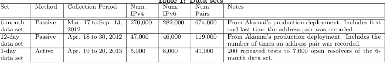
Figure 7 shows the complementary degree distribution of the vertices in the mammoth eq. class. That is, the percent of addresses (vertices) in the mammoth eq. class that are in at least a given number of pairs (edges). Figure 7 shows that the degree distribution for the IPv4 vertices is roughly the same as for the IPv6, though with a somewhat heavier tail. Although 54% of the addresses are in just one address pair, i.e. have degree one,5 as seen from the y-intercept, 8%
of the addresses are in at least 100 pairs, 4% in at least 300 pairs, and 1% in at least 500 pairs. As a comparison, for the full 6-month data set 89% of the addresses have degree one, and only 1% have degree at least 15.
AS 15169, Google, plays a major role in this mammoth eq. class.6 Although just 9% of the addresses in the mammoth eq. class are in AS 15169, 90% of the address pairs have one or both address(es) in that AS. 97% of the addresses that appear in at least 100 pairs are in AS 15169.
Whenever the IPv6 address is in AS 15169, then so is the paired IPv4. However, whenever the IPv4 address is in 15169, the paired IPv6 is not quite always in 15169 - 1% of the IPv6’s are 6to4 and another 1% are scattered across a hundred different AS’s. This is how addresses outside AS 15169 become a part of this eq. class. Some of these non-15169 IPv6 addresses may still be a part of Google’s DNS architecture, assuming that Google has deployed servers in local ISP’s with that ISP’s addresses. And also, some may be separate from GoogleDNS - if the client’s nameserver, using the public GoogleDNS for IPv4, obtained and cached the NS
5A degree one vertex in the bipartite graph does not imply
that the vertex is in a a1-1 eq. class. as the paired vertex can have degree greater than one.
6Other third-party DNS providers, such as OpenDNS and
DynDNS, are present in the data set, but to a much lesser extent compared with GoogleDNS.
0 10 20 30 40 50 1 3 10 30 100 300 1000 percent of addresses
number of pairs in which an address appears IPv4 addresses IPv4 and IPv6 addresses IPv6 addresses
Figure 7: Percent of addresses in the “mammoth” eq. class that are in at least a given number of pairs. (Complementary distribution of node degree in bi-partite graph of “mammoth” eq. class.)
Table 3: Impact on the largest equivalence class of the 6-month data set when selected address pairs are removed
After action, recompute eq. classes. Resulting largest eq. class contains:
Num of Num of Num of
Action IPv4 IPv6 addr.
addr. addr. pairs
no change to data set
8,000 9,600 247,000
omit 6to4 4,000 5,100 230,000
omit AS 15169 5,600 4,900 18,000
omit 6to4 and AS 15169
900 2,000 3,400
random subset from full data set; same num-ber of pairs as prior line
2,623±214 2,626±335 78,778±603
records returned by the first-level authoritative nameserver; and then for subsequent resolutions, sent a DNS query over IPv6 to the low-level authoritative nameserver.
6to4 addresses also play a significant role in the mammoth eq. class. Although 6to4 addresses are in only 6% of the pairs, they are 42% of the IPv6 addresses in this eq. class (an imbalance that is the opposite of AS 15169). Interestingly, for many of the 6to4 addresses, the embedded IPv4 address does not equal the observed paired IPv4. See§4.1.4 which discusses 6to4 in the full data set, not just the mammoth eq. class.
It is of interest to see what becomes the largest eq. class when, say, AS 15169 addresses are removed. Note that if one removes a set of addresses from the mammoth eq. class, the mammoth eq. class can partition into multiple smaller eq. classes - the remainder need not be a connected set of edges in the bipartite graph. Thus, we start with the full data set, and remove pairs that contain the addresses in question, and then with the reduced set of pairs, we recompute the equiv. classes and then note which is the largest one. Table 3 shows the results for selected removals.
As discussed in Section 4.1.1, some of the reduction is simply due to a smaller number of address pairs. Thus, ten random subsets from the full 6-month data set are taken, where the number of pairs in the subset is the same as in the fourth line of the Table, 225,000 pairs, down from 674,000. Given that the cases of the fourth and fifth line have the same number of pairs, their differences are due the selective removal of particular pairs, the fourth line, versus random removal. The mean value and range is reported in fifth line, and shows that the major cause for the lower complexity reported in line four is not due the smaller sample, but rather the selected pairs that are omitted.
Even with the omission of 6to4 and AS 15169, the result-ing largest eq. class still has thousands of address pairs. In§4.3 we continue the examination of largest eq. classes where we consider the 12-day data set, which has the addi-tional information of the popularity of an address pair, and we show that significant further simplification is obtained when we omit infrequently observed pairs.
4.1.4 Abnormal behavior with 6to4
Auto-tunneled [9] addresses raise a natural question whether the embedded IPv4 address (i.e. the 32 bits that come af-ter the “2002:”) matches the paired IPv4 address from the discovery technique. Somewhat surprisingly, in 63% of the pairs where the IPv6 address is 6to4, the embedded IPv4 ad-dress is different from the paired adad-dress. Overall, any 6to4 traffic is probably a bug: Given a choice between an IPv4 address and a 6to4 address, a host should always prefer IPv4 unless executing a “happy eyeballs” strategy. Since the re-solver also receives an IPv4 glue record, the rere-solver should prefer the IPv4 glue record, never attempting to connect to the DNS authority using 6to4.
Sometimes the 6to4 address is paired with hundreds of IPv4’s. For example, 2002:aca8:101::aca8:101 appears with 270 IPv4’s. The embedded address is172.168.1.1, on AOL, and located in the USA. The paired IPv4’s are mostly in Brazil, but also Germany, Saudi Arabia, and Turkey.
A likely explanation is some sort of buggy resolver soft-ware with a hardcoded 6to4 address. That we receive such 6to4 traffic also suggests that the 6to4 gateway processing this traffic isn’t validating that the embedded IPv6 address corresponds to the IPv4 address. It is not likely to be an at-tack as, if an atat-tacker took advantage of this, the query the attacker would employ would cause significantly more am-plification than the name lookups present in an Akamai-ed domain.
Also, there are stranger cases where the 6to4 is again paired with many IPv4’s but the embedded IPv4 is not routable. For example 2002:6464:64cd::6464:64cd is paired with over 250 IPv4’s and the embedded address is 100.100.100.205, or 2002:10::1:219:dbff:fef9:aa4f with embedded address 0.16.0.0. Again, this suggests buggy software misusing 6to4.
Although further investigation would be needed for a defini-tive explanation, it is clear that the collection of nameserver associations has turned out to have the additional feature of revealing abnormal activity.
Note: in calculating the percent of addresses that are in one-to-one associations,§4.1.1, we kept all of the complexi-ties in the data set, including the abnormal associations. To the extent we remove any, the percentages would just get better. 0 5 10 15 20 25 30 35 40 3 5 10 20 30 50 70 100 150200 300 500 percent of addresses
number of IPv4 + IPv6 addresses in equiv. class 200 probes 150 probes 100 probes 50 probes 40 probes 30 probes 20 probes 10 probes 1 probe
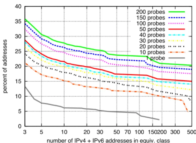
Figure 8: Percent of IPv4 + IPv6 addresses in equiv-alence classes of at least a given size, for open re-solvers probed at least 200 times on April 19-20, 2013
4.1.5 IPv4 address within IPv6 address (non-6to4)
We mention briefly that of the few, 92, pairs with Teredo IPv6 addresses, (2001:0000::/32) only one has an embed-ded IPv4 equal to the paired IPv4. Of the pairs where the IPv6 address is neither 6to4 nor Teredo, just 0.6% have an embedded IPv4 equal to the paired IPv4. Of these, 57% embed the IPv4 address in the lowest 32 bits.We also confirm an interesting human-centric convention in at least one major ISP’s DNS infrastructure that has been previously observed [16]. The operator assigns the lower 64 bits of the IPv6 address, using 16 bits to encode each octet of the IPv4 address, so that the hexadecimal values render as the decimal equivalent of the IPv4 address, such as 2001:558:1014:f:68:87:76:181. which is paired with the IPv4 address68.87.76.181.
4.2 Discovery of Complexity in Resolver
As-sociations Using Active DNS Measurements
Here, we corroborate the passively discovered complexity using the Active DNS Measurement technique of§2.2 to per-form a controlled data collection over a short time period. We first determine the open resolvers in the 6-month data set, for which we find about 7,000: 5,308 IPv4’s and 1,677 IPv6’s7. We probe each of these open resolvers via our activetechnique at least 200 times on April 19-20, 2013, request-ing resolution for our special domain which induces chains of lookups across IPv6 and IPv4 glue. Thus, we obtain a data set over a short period of time, about 13 hours, and for which the same set of nameservers is probed repeatedly. Each 4-tuple of IPv6/IPv4/IPv6/IPv4 yields either 1, 2, or 4 (IPv4, IPv6) address pairs, depending on whether the two IPv4’s and two v6’s are the same.
We are interested in the marginal benefit ofrepeated ac-tive probing of the open resolvers, from the perspecac-tive of discovering the complexity in the IPv4, IPv6 nameserver associations using a different methodology than the passive
7While there exists a much larger population of open DNS
resolvers in the Internet, we focus only on the subset of open resolvers that support IPv6 and appear within our passively collected six-month data set.
technique. We examine those resolvers for which the 4-tuple is obtained at least 200 times, and then compute equivalence classes conditioned on different amounts of probing.
Figure 8 shows the percent of addresses that are in equiv-alence classes of at least a given size, as a function of the number of probes. The curves that are higher up in the Fig-ure indicate that, overall, the equivalence classes are larger and more complex – the distribution has a heavier tail. The lowest curve in the plot is of equivalence classes of addresses from those 4-tuples discovered as a result of just the first
probe to each of the resolvers. That is, even though at least 200 probes were made, the lowest curve considers just the first one. The next curve above that one is from those 4-tuples discovered from the first ten probes, and so on. The Figure shows that with increased sampling, additional name-server addresses are discovered, and the equivalence classes overall become larger. Note that the curves are stacked on top of each other, and where the spacing varies. There is a relatively large jump between the curve for 1 probe to that of 10 probes. Then, as progressively ten more probes are incor-porated, up to 50 probes, the spacing tends to get smaller. And likewise, there is a relatively large jump between the curve for 1 probe to that of 50 probes, as compared with the incremental spacing from 50 to 100, which in turn is larger than from 100 to 150 probes, and which is about the same from 150 to 200 probes. Thus, with the additional probing, additional existing complexity is discovered, though often the marginal increase is decreasing. Moreover (and particu-larly given the impact of going from 150 to 200 probes being about the same as from 100 to 150), even after 200 probes, in all likelihood we have not discovered all of the existing complexity associated with this given set resolvers. As with the six-month data set, the largest eq. classes have addresses that span multiple continents and many AS’s.
We obtain analogous results to Figure 8 when in each eq. class, we aggregate the IPv6’s to /64 prefixes. In summary, the active DNS measurement technique also finds complex associations, even when the probing is done over a short period of time. Repeated probing reveals additional com-plexity, though the marginal increase will decrease.
4.3 Worthwhile to Record the Frequency
Ad-dress Pairs are Observed
Akamai’s initial code that aggregated the logs of the Pas-sive DNS Measurement technique did not compute a mea-sure of the frequency that an address pair was observed. Jointly with the present study, Akamai is revising the code to include this measure.
In the present section we present one application of this measure: detecting the additional complexity in nameserver associations due to address pairs that are less frequently observed.
The 12-day data set is a one-time collection from Akamai’s production deployment, and in contrast to the 6-month data set, includes the number of times an address pair was ob-served during this period. This data set is a precursor to the production deployment. The counts range from 1 to over 17 million, with a median value of 12. The pairs with highest counts belong to Comcast and ATT.
We are interested in the impact of restricting the set of address pairs to those that were observed at least 12 times in the 12 days, as well as further restrictions. We start with the full data set, and remove pairs that contain the addresses
Table 4: The 1-1 and the largest equivalence class
in the 12-day dataset, and subsets there of
% of within the largest eq cl IPv4+IPv6
Case in 1-1 Num of Num of Num of
eq cls IPv4 IPv6 pairs 12-day data set 66% 683 624 62,000 at least 12 occur-rences 78% 447 455 30,000 omit AS 15169 & 6to4 72% 346 47 764 at least 12 occur-rences; and omit AS 15169 & 6to4
82% 1 34 34
random subsets from full data set; same num of pairs as prior line
76% ± 0.7% 468 ± 5.7 508 ± 12.5 11,112 ±75.3
in question, and then with the reduced set of pairs, we re-compute the eq. classes. The results are shown in Table 4. The Table is comparable to Table 3 for the 6-month data set, and also contains aspects of Table 2.
As a sanity check, Table 4 includes info on the 1-1 eq. class. As shown in the first row, 66% of the addresses are in the1-1eq. class. This is in between the 34% for the 6-month data set, and the 71% when that data set is restricted to the final week, where the latter is more comparable in duration to present case of 12 days.
The largest eq. class contains 52% of the address pairs, which is even a greater share than the 37% of the “mam-moth” eq. class of the 6-month dataset (§4.1.3). When we omit the pairs whose addresses are in AS 15169 and whose IPv6 is 6to4, the third row, the number of pairs in the largest eq. classes is just 764, which is about 1% of what it is for the full 12-day data set, the first row. This is the same percent-age reduction as occurred with the 6-month data set, Table 3. Now, when in addition we omit pairs with fewer that 12 occurrences, the number of pairs in the largest eq. class is just 34, a further 20 fold reduction.
To distinguish from reduction due simply to a smaller number of pairs, we take ten random subsets of the full 12-day data set, where here the subsets have the same number of pairs as the fourth row of the Table 4, 21,000 pairs. The fifth row reports the mean value and range. The number of pairs in the largest eq. class is back up at 11,000, thus showing that the major cause for the relatively low com-plexity reported in line four is not due the smaller sample, but rather the selected pairs that were omitted.
4.4 Validation
To assess the IPv4 to IPv6 associations inferred via the passive DNS technique, we examine two sources of external information about the resolvers: PTRrecords and software version. Also, we were able to get feedback from three ISP’s regarding sample data.
4.4.1
PTRRecords
DNSPTRrecords map an IPv4 or IPv6 address to a human readable name. We perform a DNS PTR query for every address in the 6-month dataset. For 14.5% of the pairs, both addresses have aPTR record. For these 97,821 pairs, Table 5 shows the percent of PTR record matches for the full data set, and then partitioned by those address pairs
Table 5: Agreement between associated IPv4 and IPv6 equivalence classes and their corresponding DNS PTR records.
Set # Pairs Exact Second-Level with PTR Match Match All 97,821 4821 (4.9%) 47,752 (48.8%) 1-to-1 8461 3500 (41.4%) 5679 (67.1%) Non 1-to-1 89,360 1321 (1.5%) 42,073 (47.1%)
that are a1-1 eq. class, and those in a larger eq. class. Of the addresses in1-1 eq. classes, we see that 41% havePTR
records that match exactly, as compared to only 1.5% of the non1-1 eq. classes. IdenticalPTRrecords is supporting, though not definitive, evidence that the two addresses are either on the same server, or are the public-facing interfaces to a DNS server cluster.
Next, we examine the agreement between the IPv4 and IPv6PTR records for just the second-level domain portion of the name, e.g.foo.bar.comand faz.bar.commatch at the second-level. Whereas an exactPTRrecord match might suggest that the IPv4 and IPv6 address correspond to a common host, a load-balanced or distributed resolver might assign different hostnames to different machines, albeit with the same second-level domain. Supporting this conjecture is that while only 1.5% of the non 1-1 eq. class pairs have exactly matching PTR records, 47.1% have a second-level
PTR match. Whereas the difference is not as pronounced with pairs in1-1 eq. classes, with 41.4% matching exactly and 67.1% matching at the second-level. While DNSPTR
records are frequently incorrect or misleading, these find-ings increase our confidence that our passive technique is discovering meaningful structure.
4.4.2 Software Version
We examine the version of software reported by the DNS resolvers discovered in the eq. classes of the 6-month dataset. To ascertain the software version, we perform a DNS Chaos-net class (CHAOS)TXTtype query for the objectversion.bind. 35,921 of the addresses respond. An example response is:
“9.7.0-P2-RedHat-9.7.0-10.P2.el5_8.1”
For a baseline of what is the chance that two unrelated ad-dresses have the same version.bind, we repeatedly ran-domly pick a IPv4 and a IPv6 address from this set (ignor-ing whether or not they are observed as a pair), which yields a 3% match rate.
For 8,475 of the address pairs, both addresses return a value forversion.bind. As shown in Table 6, the version matches for 82% of these pairs, a value significantly higher than the 3% random baseline. Moreover, 99.3% of the 1-1 eq. classes have resolvers that report exactly the same version.
Together, these PTRand version.bindresults help sup-port the validity of our associations and equivalence classes. While we can not definitively ascertain whether the two ad-dresses of a pair are on the same machine, our in-progress work [8] considers other means to make a more definitive determination.
4.4.3 Feedback from Network Operators
We sent sample address associations to personal contacts at six major networks and got responses from three. All three confirmed that the IPv4 and IPv6 addresses of all of
Table 6: Agreement between associated IPv4 and IPv6 equivalence classes and their corresponding bind.version.
Set Num of Pairs with Exact bind.version Match
All 8475 6951 (82.0%)
One-to-One 4650 4619 (99.3%)
Non One-to-One 3825 2332 (61.0%)
the one-to-one associations that they checked are assigned to the same physical machine. One respondent, a cable op-erator, further explained that some of the addresses were of clients. Therefore, some of the associations we observe cor-respond to resolvers that are run on machines of customers of said cable operator.
5. DISCUSSION
This Section discusses additional details and implications of our methodology and results. In particular, we discuss the need to filter when making collocation inferences, and potential root causes for the non 1-1 eq. classes we observe.
5.1 Screening for collocated addresses
An interest in this paper is the discovery of IPv4, IPv6 address of resolvers that likely are on the same machine, or, from the viewpoint of geolocation, exist at a common loca-tion, e.g. data center. With this aim, we first wish to dis-cover the complexity that exists in the Internet of IPv4, IPv6 resolver associations, so as to avoid the false conclusion of a simple association when reality is more complicated. Our findings demonstrate that, given the complexity of address associations, the observed pairs must be filtered in order to be most valuable to higher-level objectives, e.g. geolocation. Natural candidates of value are address pairs that are in the 1-1 eq. class and have remained so over a period of time, such as six-months, or remained so after repeated, active probing, or repeated, passive observations. However, eq. classes larger than 1-1 also provide value, for instance eq. classes where the IPv6’s differ only in the lower 64 bits, given the common practice that such addresses reside on a common subnet, or may be associated with a single interface where the interface ID is varied for anonymity.
Excluding non-native IPv6 addresses is natural as these only associate the IPv4 address with the infrastructure of a particular transition strategy. If we exclude address pairs whose IPv6 is 6to4, and then compute eq. classes, and ag-gregate IPv6’s in the eq. classes to /64 prefixes, then for the six-month data set, we find that 50% of the addresses are associated with the 1-1 eq. classes of prefixes, which again is an appreciable proportion.
Having discovered address pairs that may be on the same server, we would like a technique that could make a defini-tive determination. In on-going work, we are developing an active, fingerprinting technique with that goal – see [8] for an initial description.
5.2 Large Equivalence Classes
There are several potential causes of equivalence classes larger than1-1; for DNS resolvers specifically:
• DNS queries that subvert our multi-level hierarchy, e.g. manual or automated probes from different locations directed to specific nameservers.
• Shared distributed caches, such as those commonly employed by large public DNS resolvers [15]. If NS
records returned from the first-level are saved in a shared cache (with TTL of 12 hours for the present data set) and subsequently used by another resolver that sends a query over IPv6, then the second-level will discover multiple IPv6’s associated with a single IPv4. A short TTL on the final AorAAAArecord (20 seconds in the data set) increases reuse of the cached
NSrecord. Furthermore, after theNSTTL expires and some other resolver using the shared cache does the lookup at the first-level, then another IPv4 address could be added to the equivalence class.
However, our results offer a more general caution in efforts that attempt to pair IPv4 and IPv6 addresses. Complicat-ing factors that contribute to the complexity observed in our data, but are not specific to DNS and may affect other measurement efforts, include:
• Hosts and interfaces with multiple IPv4 and/or IPv6 addresses.
• Network Address Translation (NAT) [29] of either IPv4 or IPv6, where we observe multiple addresses of the non-translated protocol that correspond to a smaller set of addresses from the other. Such translation may occur at the edge, or within the carrier [20].
• Other forms of middleboxes, including load balancers, e.g. [3].
• Auto-tunneling, including 6to4, Teredo, etc [9]. • Address changes over time, including ephemeral
ad-dresses [31] and IPv6 privacy extensions [24].
6. CONCLUSIONS
This paper seeks to characterize the inter-relation of IPv4 and IPv6 among Internet DNS resolvers. We deploy both active and passive measurement techniques to discover and analyze sets of associated pairs of IPv4, IPv6 addresses.
While prior work has examined IPv4, IPv6 associations for clients, to our knowledge this paper is the first to begin to examine such associations for equipment within operators’ networks, which can be a leading indicator of IPv6 adoption [12, 1].
We develop and deploy two novel measurement systems: i) a passive, opportunistic technique using a two-level DNS hi-erarchy that encodes IPv4 addresses within IPv6 nameserver records; and ii) an active DNS probing system that induces a combination of IPv4 and IPv6 DNS resolver lookups in a single resolution operation.
For a six-month passive data collection, we find that 34% of the addresses have a one-to-one association, i.e. appear in no other address pair. This percentage increases to al-most 50% when the IPv6’s are aggregated to /64’s. We consider this a positive result for finding candidate address pairs that likely are on the same server or subnet, and are collocated. Supporting evidence is provided via matching PTR records and software versions, and confirmation from three major Network Operators of sample pairings. Com-panion, in-progress work seeks to develop a fingerprinting technique that would confirm whether an address pair is on the same server, [8].
In contrast to such simple associations, we also find com-plex, connected sets of address pairs that, at the extreme, span continents and hundreds of ASes, where third-party resolvers with distributed shared caches [15] play a major role. We also observe multiple instances of abnormal use of 6to4 tunnels, where a 6to4 address is paired with hundreds of different IPv4’s that again span multiple continents, and where the IPv4 embedded in the 6to4 does not equal any of the paired IPv4’s.
The active technique, which was designed, implemented, and deployed completely separately from the passive one, also discovers significant complexity on the address-pair as-sociations. It did so in the context of a controlled experiment of repeated probing of a given set of open resolvers over a short period of time, 13 hours.
The passive technique has been implemented in Akamai Technologies’ DNS infrastructure, where the collected pairs, after appropriate filtering, are being used to bootstrap ge-olocation of IPv6 addresses, and were helpful for revisions to request-routing software to handle IPv6.
Acknowledgments
Matthew Levine had the original idea for the opportunistic nameserver technique, while Steve Hill, James Kretchmar, and Brian Sniffen contributed to its design and implemen-tation at Akamai Technologies. Patrick Gilmore provided insights into common practice of network operators, and via his contacts obtained feedback on sample address pairs. Our shepherd, John Heidemann, helped to review and properly frame the work. Thanks to the anonymous reviewers, Mark Allman, Billy Brinkmeyer, Aaron Hughes, and Geoffrey Xie for invaluable feedback on initial drafts of this work. This work supported in part by NSF grants 1111445, CNS-1111672, and CNS-1213157. This material represents the position of the authors and not necessarily that of the NSF, Akamai Technologies, or the U.S. Government.