HAL Id: lirmm-02045144
https://hal-lirmm.ccsd.cnrs.fr/lirmm-02045144
Submitted on 21 Feb 2019
HAL
is a multi-disciplinary open access
archive for the deposit and dissemination of
sci-entific research documents, whether they are
pub-lished or not. The documents may come from
teaching and research institutions in France or
abroad, or from public or private research centers.
L’archive ouverte pluridisciplinaire
HAL
, est
destinée au dépôt et à la diffusion de documents
scientifiques de niveau recherche, publiés ou non,
émanant des établissements d’enseignement et de
recherche français ou étrangers, des laboratoires
publics ou privés.
Parallel Computation of PDFs on Big Spatial Data
Using Spark
Ji Liu, Noel Moreno Lemus, Esther Pacitti, Fábio Porto, Patrick Valduriez
To cite this version:
Ji Liu, Noel Moreno Lemus, Esther Pacitti, Fábio Porto, Patrick Valduriez. Parallel Computation
of PDFs on Big Spatial Data Using Spark. Distributed and Parallel Databases, Springer, 2020, 38,
pp.63-100. �10.1007/s10619-019-07260-3�. �lirmm-02045144�
Ji Liu · Noel Moreno Lemus · Esther Pacitti · Fabio Porto · Patrick Valduriez
the date of receipt and acceptance should be inserted later
Abstract We consider big spatial data, which is typically produced in scientific areas such as geological or seismic interpretation. The spatial data can be produced by observation (e.g.using sensors or soil instruments) or numerical simulation programs and correspond to points that represent a 3D soil cube area. However, errors in signal processing and modeling create some uncertainty, and thus a lack of accuracy in identifying geological or seismic phenomenons. Such uncertainty must be carefully analyzed. To analyze uncertainty, the main solution is to compute a Probability Density Function (PDF) of each point in the spatial cube area. However, computing PDFs on big spatial data can be very time consuming (from several hours to even months on a computer cluster). In this paper, we propose a new solution to efficiently compute such PDFs in parallel using Spark, with three methods: data grouping, machine learning prediction and sampling. We evaluate our solution by extensive experiments on different computer clusters using big data ranging from hundreds of GB to several TB. The experimental results show that our solution scales up very well and can reduce the execution time by a factor of 33 (in the order of seconds or minutes) compared with a baseline method.
Keywords Spatial data·big data·parallel processing·Spark
1 Introduction
Big spatial data is now routinely produced and used in scientific areas such as geological or seismic interpretation [10]. The spatial data are produced by observation, using sensors [46], [12] or soil instruments [25], or numerical simulation, using mathematical models [15]. These spatial data allow identifying some phenomenon over a spatial reference [19]. For instance, the J. Liu
Inria and LIRMM, Univ. of Montpelier, France E-mail: [email protected] N. Moreno Lemus
LNCC Petr´opolis, Brazil E-mail: [email protected] E. Pacitti
Inria and LIRMM, Univ. of Montpelier, France E-mail: [email protected] F. Porto
LNCC Petr´opolis, Brazil E-mail: [email protected] P. Valduriez
Fig. 1:The distribution of a point.
spatial reference may be a three dimensional soil cube area and the phenomenon a seismic fault, represented as quantities of interest (QOIs) of sampled points (or points for short) in the cube space. The cube area is composed of multiple horizontal slices, each slice having multiple lines and each line having multiple points. A single simulation produces a spatial dataset whose points represent a 3D soil cube area.
However, errors in signal processing and modeling create some uncertainty, and thus a lack of accuracy when identifying phenomenons. Such uncertainty must be carefully quantified. In order to understand uncertainty, several simulation runs with different input parameters are usually conducted, thus generating multiple spatial datasets that can be very big,e.g.hundreds of GB or TB. Within multiple spatial datasets, each point in the cube area is associated to a set of different observation values. The observation values are captured by sensors, or generated from simulation, at a specific point of the spatial area.
Uncertainty quantification of spatial data is of much importance for geological or seismic scientists [34], [45]. It is the process of quantifying the uncertainty error of each point in the spatial cube space, which requires computing a Probability Density Function (PDF) of each point [26]. The PDF is composed of the distribution type (e.g.normal, exponential) and necessary statistical parameters (e.g.the mean and standard deviation values for normal and rate for exponential).
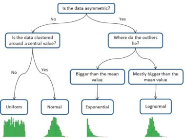
Figure 1 shows that the set of observation values at a point may be modelled by four distri-bution types,i.e.uniform (a), normal (b), exponential (c), and log-normal (d). The horizontal axis represents the values (V) and the vertical axis represents the frequency (F). The green bars represent the frequency of the observation values in value intervals and the red outline represents the calculated PDF. Given a resulting PDF modeling the data distribution at a point, there may be some error between the distribution of the observation values and one produced by a PDF. During the process of fitting data to a PDF, we aim at reducing such PDF error (or error for short in the rest of the paper) to a minimum. For instance, the set of observation values corresponding to the QOI at a point obeys a normal distribution shown in Figure 1 (b). The mean value of the set of observation values (see Equation 1) may be used as a representative of QOI since it has the highest chance to be the QOI. However, the distribution can be different from normal. And analyzing uncertainty just using the mean or standard deviation values is difficult and imprecise. For instance, if the distribution type of simulated values is exponential (see Figure 1 (c)), we should take the value zero (different from the mean value of the simulated values) as the QOI value since it has the highest frequency. Thus, once the PDF of observations in a point has been computed, we can calculate the QOI value that has the highest probability. The QOI value can be assumed to represent the imprecision among the point observations, and computed across the whole spatial dataset as a measure of point observations uncertainty.
Calculating the PDF that best fits the observation values at each point can be time consum-ing. For instance, one simulation of an area of 10km (distance) * 10km (depth) * 5km (width) corresponds to 2.4 TB data with 10000 measurements at each point [2]. This area contains 6.25 * 108 points. The time to calculate the PDF with consideration of 4 distribution types (normal,
uniform, exponential and log-normal) can be up to several days or months using a computer cluster (or cluster for short).
The problem we address is how to efficiently compute PDFs under bounded error constraints. There are three main challenges,i.e.big data, long and complex computation and error bound. First, the input spatial datasets can be very big. Imagine that the size of each spatial dataset is several hundred MB, then 10,000 spatial datasets correspond to several TB, which makes it hard to process. Second, computing PDFs is complex and takes time. The PDF computation with the datasets of several TB in a single computer or a small cluster (6 nodes, each with 32 CPU cores) may take up to several months. Third, the PDF computation should not have unacceptable error, i.e.under error bound. For instance, if the error is bigger than 50%, then the result will not be representative.
Solutions for computing PDFs are now available in popular programming environments for numerical and statistical analysis, such as MATLAB and R. MATLAB provides libraries [31][36] that use a baseline method for PDF fitting. R provides the GLDEX library that supports the Generalized Lambda Distribution (GLD) family of PDFs. However, these implementations do not address the problem of efficient computation of thousands or millions of PDFs that may lead to redundant computation. Machine Learning (ML) techniques are widely used to process big data [4, 14] for the sake of prediction and classification [44]. They can be used for reducing the dimension of data [24], reducing the time for repeating work [8] and discovering knowledge based on big data [21]. However, unlike the traditional approach, we do not use ML to reduce the data dimension. Instead, we use ML to discover new knowledge in order to reduce redundant computation of PDFs. Furthermore, we use data aggregation to reduce the quantity of data to process.
In this paper, we propose a new solution to efficiently compute PDFs in parallel using Spark [49], a popular in-memory big data processing framework (see [29] for a survey on big data systems). The main reason to choose Spark is that, unlike MPI, it makes it easy to parallelize application code in a cluster. Futhermore, it makes efficient use of main memory to deal with intermediate data (RDD) that is used repeatedly, as with ML algorithms. In addition to deploying PDF computation over Spark, we propose three new methods to efficiently compute PDFs: data grouping, ML prediction and sampling. Data grouping consists in grouping similar points to compute the PDF. In the original input data, the data corresponding to some points may be the same or very similar to the data corresponding to a common point. ML prediction uses ML classification methods to predict the distribution type of each point. Sampling method enables to efficiently compute statistical parameters of a region by sampling a fraction of the total number of points to reduce the computation space.
To validate our solution, we use the spatial data generated from simulations based on the models from the seismic benchmark of the HPC4e project between Europe and Brazil for oil and gas exploration [2]. This benchmark includes MATLAB models for seismic wave propagation. In oil and gas exploration, seismic waves are sent deep into the Earth and allowed to bounce back. Geophysicists record the waves to learn about oil and gas reservoirs located beneath Earth’s surface.
This paper makes the following contributions:
– A scalable approach and architecture to compute PDFs of QOIs in large spatial datasets
using Spark;
– Three new methods to reduce the time of computing PDFs,i.e.data grouping, ML prediction and sampling;
– An extensive experimental evaluation based on the implementation of the methods in a
results show that our methods scale up very well and reduce the execution time by a factor of 33 (in the order of seconds or minutes) compared with a baseline method;
The three new methods,i.e. data grouping, ML prediction and sampling, are the main contri-butions of the paper. In addition, the layered architecture and the optimization methods (see details in Section 5.2) are also contributions for the basic processing of PDFs. The architecture is deployed in the execution environment and the optimization methods are directly implemented in a Scala program, thus facilitating the use of the three new methods.
The paper is organized as follows. Section 2 discusses related work. Section 3 introduces some background on Spark. Section 4 gives the problem definition. Section 5 presents our architecture for computing PDFs with Spark, with its main functions. Section 6 presents our solution to compute PDFs in parallel, with three methods,i.e.data grouping, ML prediction and sampling. Section 7 presents our experimental evaluation on different clusters with different data sizes, ranging from hundreds of GB to several TB. Section 8 concludes.
2 Related work
The importance of modeling data distribution through PDFs have been acknowledged in various domains such as seismology, finance, meteorology or civil engineering [11, 47]. There is variability in almost any value that can be measured by observation and almost all measurements are made with some intrinsic error. Thus, simple numbers are often inadequate for describing a quantity, while PDFs are more appropriate. As the number of observations increases, efficient techniques to fit a set of observations to a PDF become paramount in practical applications [13, 17, 6]. For instance, the fitdistr function, which implements the Maximum Likelihood Estimation (MLE) (for normal, log-normal, geometric, exponential and Poisson distributions) and Nelder-Mead (NM) [35] (for the other distributions) methods in R [1], calculates the PDF with small error for a given PDF type. This function scans the input data once and the time complexity of both methods isO(n), withninput observation values for the same point [42].
In this paper, we are interested in situations where large number of observations of the same quantity of interest are registered in thousands or even millions of spatial positions. This is the case, for instance, in numerical simulations that compute the values of QOIs through a set of points that discretizes a physical domain, e.g. representing the subsurface of the ocean in a seismic simulation. In this context, Campisano et al. [9] model series of observations at spatial positions in a grid as spatial-time series. The model helps supporting predictions on QOIs. This work is orthogonal to ours, as we strive to inform about the uncertainty exhibited by observations drawn from a continuous domain of values through a spatial region, which can be obtained by fitting the distribution to a PDF.
Another approach adopts the Generalized Lambda Distribution (GLD), a function for model-ing a family of distributions [37], such as: normal,uniform, exponential, lognormal, gamma, etc., usingλparameters, represented asGLD(λ1, λ2, λ3, λ4). The lambda parameters specify the loca-tion, scale and both sides of the tail of distributions, respectively, thus making it general enough to cover a variety of distributions. This generality of the GLD function is particularly interesting to avoid testing for a best fit among possible PDF function types. GLDs however cover a space of values in theλ3andλ4parameter space while being invalid in some other regions. Thus, when the distribution of a certain set of observation values is not covered by the space ofλ3andλ4, the GLD error can be very big. Therefore, for some distributions, the GLD approach may not offer a good fit, or even none at all. Moreover, there are a handfull of parameter estimation (i.e.data fitting) techniques, such asMaximum log-likelihood [5]. Theses techniques solve an optimization problem that starts from a random initial parametrization and numerically integrates the space
of probabilities minimizing, for example, the squared error, between the GLD and the set of observations. Therefore, for very large number of points (i.e.sets of observations) for which we may want to compute the corresponding GLD, specifying strategies that reduce the number of fitting computations is still needed and is the focus of this work.
In order to tackle the redundant PDF computation problem, we apply ML techniques. ML is now widely used to process big data [4, 14] in activities such as regression analysis and classi-fication [44, 40]. It has been used to reduce the number of redundant computation by clustering data and reducing data dimensions to detect parameter dependent structures [8] or discover knowledge out of big data [21]. More recently, ML has been used as substitutes for traditional data structures in database systems, such as B+ tree indexing and caching [27].
Considering that fitting thousands or millions of sets of observations to PDF functions is a daunting task, we use ML to save total computation cost and reduce fitting elapsed time. In particular, we use the unsupervised k-means algorithm [33] to cluster similar sets of observations and the decision tree supervised algorithm to classify the distribution types using the mean and variance statistical moments of known observation sets with associated PDF types as training data [20].
3 Background on Spark
Spark [49] is an Apache open-source data processing framework. It extends the MapReduce model [16] for two important classes of analytics applications: iterative processing (machine learning, graph processing) and interactive data mining (with R, Excel or Python). Compared with MapReduce, it improves the ease of use with the Scala language (a functional extension of Java) and a rich set of operators (Map, Reduce, Filter, Join, Aggregate, Count, etc.). In Spark, there are two types of operations: transformations, which create a new dataset from an existing one (e.g.Map and Filter), and actions, which return a value to the user after running a computation on the dataset (e.g.Reduce and Count). Spark can be deployed on shared-nothing clusters, i.e.clusters of commodity computers with no sharing of either disk or memory among computers. In a Spark cluster, a master node is used to coordinate job execution while worker nodes are in charge of executing the parallel operations.
Spark provides an important abstraction, called resilient distributed dataset (RDD), which is a read-only and fault-tolerant collection of data elements (represented as key-value pairs) partitioned across the nodes of a shared-nothing cluster. RDDs can be created from disk-based resident data in files or intermediate data produced by transformations. They can also be made memory resident for efficient reuse across parallel operations.
Spark data can be stored in the Hadoop Distributed File System (HDFS) [41], a popular open source file system inspired by Google File System [22]. Like GFS, HDFS is a highly scalable, fault-tolerant file system for shared-nothing clusters. HDFS partitions files into large blocks, which are distributed and replicated on multiple nodes. An HDFS file can be represented as a Spark RDD and processed in parallel.
Spark provides a functional-style programming interface with various operations to execute a user-provided function in parallel on an RDD. We can distinguish between operations without shuffling, e.g. Map and Filter, and with shuffling, e.g. Reduce, Aggregate and Join. Shuffling is the process of redistributing the data produced by an operation, e.g. Map, so that it gets partitioned for the next operation to be done in parallel,e.g. Reduce. This process is complex and expensive and requires moving data across cluster nodes.
In this paper, we exploit Spark MLlib [3], a scalable machine learning (ML) library that can handle big data [28] in memory by exploiting Spark RDDs and Spark operations. In one method
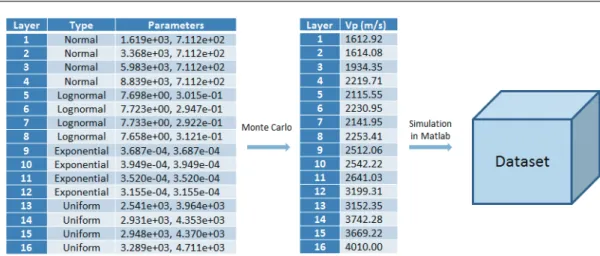
Fig. 2:Data generation from simulation.This process is repeated multiple times in order to generate multiple datasets. The values ofV pare different at different iterations.T yperepresents the distribution type.
which we propose, we use ML techniques to classify the distribution types of the observation values at different points in order to reduce useless calculation.
4 Problem Definition
In this section, we first present how we generate the spatial datasets, which is the input for the problem. Then, we present the challenges to process the big input data. Afterwards, we present the problem in details.
4.1 Spatial Dataset Generation
A spatial dataset contains the information to generate an observation value matrix that corre-sponds to a three dimensional cube area. As a result of running multiple simulations, multiple spatial datasets are produced with a set of observation values at each point. The set of observa-tion values at each point enables the computaobserva-tion of their mean value, standard deviaobserva-tion values and PDF.
Let us illustrate the problem with the spatial data generated from simulations based on the models from the seismic benchmark of the HPC4e project [2]. An important parameter of the models is wave phase velocity, notedV pin electromagnetic theory, which is the rate at which the phase of the wave propagates in space. The models contain 16 layers and each layer is associated to a value ofV p. The top layer delineates the topography and contains the description information of the other 15 layers. Each of the 15 layers is used to generate the observation values of points in a horizontal space of the cube area. A set of 16 layers can generate a spatial dataset, where each point corresponds to an observation value. Then,N sets of 16 layers can generateN spatial datasets, where each point corresponds to a set ofN observation values.
Since our purpose is to study the uncertainty in the output as a result of the wave propagation of the input uncertainty through the model, we assume that the input value of each layer is uncertain and obeys a PDF. The distribution types for every four layers are: Normal (for the
first four layers), Log-normal (for the fourth to eighth layers), Exponential (for the ninth to twelfth layers) and Uniform (for the rest). We use a Monte Carlo method to generate different sets of the 16 input parameters. For each set of input parameters, we generate a spatial dataset using the models as shown in Figure 2. In Figure 2, we use the Monte Carlo method to generate a set of 16 variables, each of which corresponds to the V pof each layer. Then, we execute the MATLAB programs of the seismic benchmark to generate a spatial dataset. Finally, we repeat this process multiple times in order to generate multiple datasets.
4.2 Challenges
Computing PDFs on spatial datasets raises three main challenges,i.e.big data, long and complex computation and error bound.
First, as the input spatial datasets can be very big, a simple scan of the input data is not enough. After scanning the data, we need to perform a join operation to merge the observation values of each point with a set of observation values. This join operation may take much time when there are many points. Since the data corresponding to the same point are distributed at different nodes in a cluster, the join operation requires shuffling, which may take much time. In addition, when the input data is very big, we cannot cache all the data in memory.
Second, computing PDFs is complex and takes time for big spatial datasets. In order to calculate the PDF of a point, we use the fitdistr function, which implements MLE and NM method (a commonly used and robust numerical method) in an R program. The fitdistr function optimizes a cost function using multiple iterations, which may take much time. In addition, this function is only used for calculating the PDF of a single point, which takes a vector of observation values as input and calculates the PDF of a specific distribution type. Furthermore, this function is designed for execution in a single machine, and is not scalable for a cluster environment. In our problem, we need to first extract the observation values of each point from a spatial dataset. Then, for each point, we must calculate the PDF of an appropriate type, which corresponds to the minimum error. Finally, the results must be stored in a file system. This complex process can take much time with a basic approach. For instance, with a cluster of 6 nodes, each with 32 CPU cores, it takes about 63 days using the baseline method (see details in Section 6.1) and the fitdistr function in R language to compute the PDFs of all the points in all the slices of a cube with a dataset of 2.4TB. Thus, computing PDFs is complex and takes time for big spatial datasets.
Third, the PDF computation should not have unacceptable error, i.e. under error bound. For instance, if the error is bigger than 50%, then the result will not be representative. This requirement implies choosing a distribution type that corresponds to the minimum error. The fitdistr function in the R program can only fit the parameters corresponding to a specific distri-bution type to calculate the PDF based on a set of observation values. But it cannot choose a distribution type.
4.3 Problem Formulation
The main problem we address is to efficiently compute PDFs on big spatial datasets, such as the seismic simulation data discussed above. Since it takes much time to compute the PDFs of the points in the whole cube area, our approach is to divide it into multiple spatial regions and compute the PDFs of all the points in a chosen region within a reasonable time. The spatial region is chosen based on some statistical parameters of the region. Thus, the main problem is how to efficiently calculate the PDF of each point in a spatial region,e.g.a horizontal slice in the cube
area, with a small average error between the PDF and the distribution of the observation values. A slice is a set of points that correspond to the same position in one of the three dimensions. In order to choose a region, the mean and standard deviation values and the distribution type of a part of the points in the spatial region should be computed. In addition, the average mean value, the average standard deviation value and the percentage of points corresponding to each distribution type in all the points of the region can also be computed. We denote these statistical parameters of a spatial region to compute by the features of a spatial region. A related subproblem is how to efficiently calculate the features of a spatial region. In this paper, we take a horizontal slice as a spatial region.
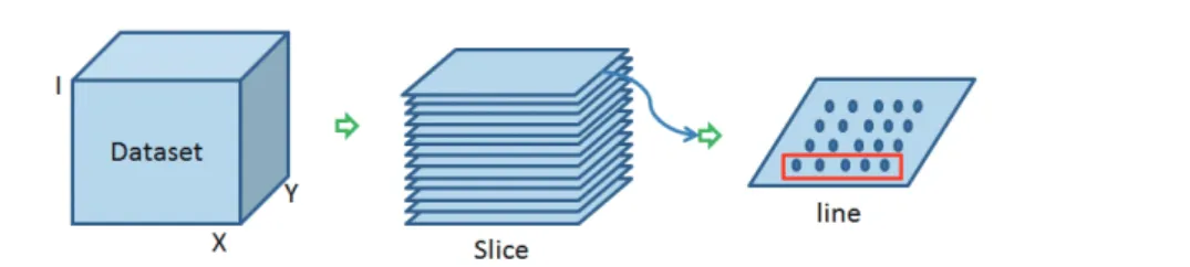
The input data is the set of spatial datasets, which are generated from the simulation as explained in Section 4.1. LetDSbe a set of spatial datasets,dbe a spatial dataset inDS andN be the number of points in a slice (the same for Equations 3, 4 and 6).dis generated using a set ofV pof the 16th layers (each set ofV pis different). As shown in Figure 3, eachdis composed of a matrix of observation values corresponding to the sampled points in the cube area.X, Y, Irepresent the first, second and third dimensions of the cube area and the index of observation values in the dataset. In the spatial data domain, the first dimension (x) is inline; the second dimension (y) is crossline and the third dimension (i) is time or depth. A dataset is composed of multiple slices, and each slice is composed of multiple lines. Each slice corresponds to the same position in the third dimension (I), and each line corresponds to the same position in the second (Y) and third (I) dimensions. In this paper, we take a slice (i.e.Slice 201 in Section 7) as the region to calculate PDFs. Each point (px,y,i) is represented as an observation value in the
dataset and the indices arex,yandiin each dimension. Based on multiple datasets, each point px,y in Sliceicorresponds to a set of valuesV ={v1, v2, ..., vn}whilevk is the observation value
corresponding to the pointpx,y in Slicei indk∈DSandnis the number of observation values
in the set (the same for Equations 1, 2 and 5).dk represents thekth dataset (d) inDS.
Based on these notations, we define Equations 1 - 4 and 6, which are based on the formulas in [18]. The mean (µx,y) and standard deviation (σx,y) values of a point can be calculated according
to Equations 1 and 2, respectively. And the average mean (µi) and standard deviation (σi) values
of Sliceican be calculated according to Equations 3 and 4, respectively. The errorex,y,ibetween
the PDFF and the set of observation valuesV can be calculated according to Equation 5, which compares the probability of the values in different intervals inV and the probability computed according to the PDF. The intervals are obtained by evenly splitting the space between the
maximum value and the minimum value in V. min is the minimum value in V, max is the
maximum value in V and L represents the number of all considered intervals, which can be
configured.F reqk represents the number of values inV that are in thekth interval. The integral
of P DF(x) computes the probability according to the PDF in the kth interval. Equation 5 is inspired by the Kolmogorov-Smirnov Test [30], which tests whether a PDF is adequate for a dataset. In addition, we assume that the probability of the values outside the space between the maximum value and the minimum value is negligible for this equation. Then, the average error E of Slicei can be calculated according to Equation 6.
µx,y =
Pn
i=1vi
n (1)
σx,y=
s
Pn
i=1(vi−µ)2
n−1 (2)
µi=
P
px,y∈sliceiµx,y
Fig. 3:Dataset structure. A dataset is composed of multiple slices. Each slice is composed of multiple lines. The red rectangle represents a line. Each circle represents a point, which contains an observation value of the point in the original cube area.
σi =
P
px,y∈sliceiσx,y
N (4)
ex,y,i= L
X
k=1
| F reqk
n −
Z min+(max−min)∗Lk
min+(max−min)∗k−1
L
P DF(x)dx| (5)
E=
P
px,y∈sliceiex,y,i
N (6)
We can now express the main problem as follows: given a set of spatial datasets DS =
{d1, d2, ..., dn} corresponding to the same spatial cube area C ={slice1, slice2, ..., slicej}, how
to efficiently calculate the mean, standard deviation values and the PDF F at each point in slicei ∈Cwith a small average errorEnot higher than a predefined average errorε. In addition,
we also need to compute the statistical parameters of slices in order to choose Sliceimentioned in the first subproblem. Thus, the related subproblem can be expressed as: how to efficiently calculate the features of a slice when given the same datasetsDS. The features are:
– µ,σand distribution type of some points in the slice
– µi,σi and the percentage of points for each distribution type in all the points of the slice
5 Architecture for Computing PDFs
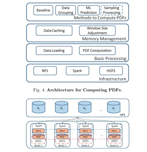
In this section, we describe the architecture for PDF computation (see Figure 4). This architecture has four layers, i.e. infrastructure, basic process to compute PDFs, memory management and methods to compute PDFs. The higher layers take advantage of the lower layers’ services to implement their functionality. The infrastructure layer provides the basic execution environment, including Spark, HDFS and Network File System (NFS) in a cluster. The basic processing layer provides guiding principles to load the big spatial data and to compute PDFs. The memory management layer allows optimizing the execution of the basic process by caching data and managing tumbling windows on big data. The methods to compute PDFs are presented in Section 6.
The architecture has four layers and decomposes the problem in smaller problems, which can be solved independently and efficiently. In each layer, we use different optimization methods, e.g. data caching, window size ajustement, parallel data loading, to speed up execution. As a result, the baseline approach (see details in Section 6.1) also benefits from our architecture, which explains why it yields relatively good performance and good scalability.
Fig. 4:Architecture for Computing PDFs.
Fig. 5:Infrastructure. di represents theith spatial dataset.
5.1Infrastructure with Spark
Figure 5 illustrates the infrastructure we deploy to process big spatial data. The big spatial data is produced by simulation application programs and stored in NFS [39], a shared-disk file system that is popular in scientific applications. Spark and HDFS are deployed over the nodes of the cluster. The intermediate data produced during PDF computation and the output data are stored in HDFS, which provides persistence and fault-tolerance.
Keeping the input spatial data in NFS allows us to maximize the use of the cluster resources (disk, memory and CPU), which can be fully dedicated for PDF computation. With the input data stored in NFS, the NFS server is outside the Spark/HDFS cluster and takes care of file management services, including transferring the data that is read to the cluster nodes. An al-ternative solution would have been to store the input data in HDFS, which would lead to have HDFS tasks competing with Spark tasks for resource usage on the same cluster nodes. We did try this solution and it is much less efficient in terms of data transfer between cluste nodes. This is because HDFS is more complex and does more work due to fault-tolerance and data replication. Note that we use NFS only for data loading (see Algorithm 2), while the data generated from execution is persisted in HDFS.
We use Spark as our execution environment for computing PDFs. We developed a program written in Scala, which realizes the functionality of different methods to compute PDFs. Once the method to compute PDFs is chosen, the Scala program is executed as a job within Spark.
5.2Principles for the Basic Processing of PDFs
The basic processing of PDFs consists of data loading, from NFS to Spark RDDs, followed by PDF computation using Spark. The data loading process treats the data corresponding to a slice and pre-processes it,i.e.calculates statistical parameters of observation values of each point and relates the observation values of each point to an identification of the point. The identification of each point is an integer value which represents the location of the point in the cube area. Then, the PDF computation process groups the data and calculates the PDFs and errors of all the points in a slice based on the pre-processed data. To make the basic processing of PDFs efficient, we use the following guiding principles.
1. Parallel data loading. To perform data loading in parallel, we store the identifications of points in an RDD, which is evenly distributed on multiple cluster nodes. For each point in a node, all the corresponding values in different spatial datasets are retrieved from NFS. At the same time, the mean and standard deviation values are calculated. Then, the identification of the point is stored as the key of the point. The mean and standard deviation values and the observations values are stored as the value of the point. The key and value of the point are stored as a key-value pair in the RDD. This loading process is realized by a Map operation in Spark, which is fully parallel.
2. Data grouping. In order to avoid repeating the PDF computation for the same or similar sets of observation values, we group the data of different points that shares similar statistical features, e.g. the mean and standard values. Then, a representative point of the group is chosen. The PDF of the representative point is taken to represent all the points in the group. Thus, the PDF computation of all the points in the group is reduced to the computation of the representative point. The grouping can be realized using an Aggregation operation in Spark. However, the shuffling process in the Aggregation operation may take much time. When this occurs, then we can simply avoid data grouping. To decide whether to use data grouping, the ideal solution would be to have a cost model, but it is difficult to estimate the time to transfer data within Spark. However, we can test if data grouping is effective on small workloads,e.g.a few lines of points in a slice as explained in Section 7.
After data grouping, the set of the identifications of the points in the group is stored as a part of the value in the key-value pair. For each representative point, the key represents the identification while the value contains the mean and standard deviation values and the observation values.
3. Parallel processing of PDFs. The PDF of each point (or representative point) is computed based on its observation values. This process is also realized in a Map operation, which distributes the key-value pairs in RDD of different points to different nodes. There are two
methods to calculate the PDF of a point, i.e. with ML and without ML. With ML, the
distribution type corresponding of a point is predicted (see Section 6.3 for more details), and then the PDF and error,i.e.PDF error, are computed. Without ML, the PDFs of different distribution types are computed, and the PDF of the minimum error is chosen as the PDF of the point. The PDF computation of different points is executed in parallel in different nodes of the cluster. After the parallel processing of PDFs, the key remains the identification of each point (representative point) while the PDF is stored as a part of the value in the key-value pair of the RDD. In addition, since the mean and standard deviation values and
the observation values are no longer useful, the corresponding data is removed from the value in the key-value pair. Finally, the PDF of each point is persisted in a file or database system for future use. In addition, an average error of the PDF of the points in the slice is calculated and shown as the result of executing the Scala program.
4. Tumbling window.Since a slice can have many points that won’t fit in memory, we use a tumbling window over the slice during data loading, data grouping and parallel processing of PDFs. A window represents a set of points to process, which corresponds to a swath area of several continuous lines in the slice to process. Any two windows have no intersection. After the processing of one window, the process of the next window begins until the end of the slice. Once the size of the window is configured, it stays the same during execution. The size of the window has strong impact on execution and must be chosen carefully (see details in Section 5.3.2). Note that the tumbling window is different from the data chunk in Spark. Data chunk is generated by splitting the data in RDD, which is stored in each node of the cluster node. The window here is a unit of points to process by all the nodes in the cluster.
5. Use of external programs. In the parallel data loading and parallel processing of PDFs, we use external programs, which do the specific loading of the points. Since some Java functions, e.g. skipBytes (Skips and discards a specified number of bytes in the current file input stream), may not work correctly during the parallel execution of a Map operation in Spark [23], we call an external Java program in the Map operation to retrieve observation values of a point from different spatial datasets and pre-process values. Since the PDF computation is implemented by an external program (in R), we call it within the Map operation for the parallel processing of PDFs. Finally, the output data of the external program is transformed to key-value pairs and stored in RDDs by the same Map operation, which executes the external program.
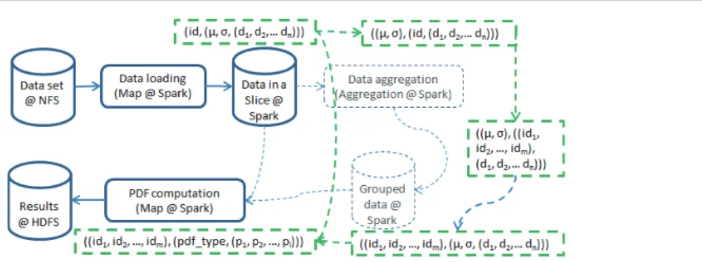
Figure 6 shows the data flow of the process. First, the data is loaded from NFS in parallel. The data is stored in an RDD; the key is the identification (id) of each point and the value is the set of the mean and standard deviation value and the observation values of each point. Theidof each point is calculated based on its indices in the three dimensions. If we apply data grouping, the key value pairs are processed in three steps. First, we take the mean and standard deviation value as the key and put theid and the set of observation values of each point as value. Then, the RDD is grouped based on the key,i.e.the mean and standard deviation values. The set of idof the points of the same group is stored in the value. In addition, we store the first set of the observation values in the value. Then, we take the set ofidas the key, and the mean value, the standard deviation value and the set of observation values as the value. If we do not apply data grouping, we have only oneidin the key. We calculate the PDF based on the set of observation values. Finally, we have the set ofidas key and the PDF type and the PDF parameters as value, which is stored in HDFS.
5.3Memory Management
In order to efficiently compute PDFs, we use two memory management techniques to optimize the calculation of PDFs over big data: data caching and window size adjustment.
5.3.1Data Caching
We use data caching, i.e. keeping data in main memory, to reduce disk accesses. To identify which data to cache, we distinguish between four kinds of data: input data, instruction data, intermediate data and output data. The input data is the original data to be processed,i.e.the
Fig. 6:Data flow and key value pairs. The blue boxes and arrows represent the data flow. @Spark represents that the data is stored in a Spark RDD. The green boxes and arrows represent key value pairs corresponding to the data flow.id represents the id of each point. A set ofd1 to dn represents the observation values.µandσrepresent the mean and standard derivation value
of the set of observation values. The set ofid1 to idmrepresents the ids of all the points in the
group after data grouping. If data grouping is not used, there is only one id as the key of the key value pair in the result of the PDF computation.pdf typerepresents the type of PDF. The set ofp1 topl represents the parameters of the calculated PDF.
big spatial datasets. The instruction data is the data corresponding to the external programs, e.g.Java or R programs used in data loading and PDF computation. The intermediate data is the data generated by the data loading process or the execution of external programs, and used by subsequent execution. The output data is the final data generated by the PDF computation. We use a simple caching strategy. We do not cache input data because it can be very big and read only once. We only cache instruction data and intermediate data, which are accessed much during execution. However, intermediate data that is not used in subsequent operations is removed from main memory. The output data is written to memory first and then persisted.
During execution, some intermediate data that is stored in Spark RDDs can be cached using
the SparkCacheoperation, which stores RDD data in main memory. However, the instruction
data of external programs and the intermediate data directly generated by executing these ex-ternal programs are outside of RDDs. We cache this data in temporary files in memory, using a memory-based file system [43]. Then, the information in the cached files is retrieved and stored as intermediate data in RDDs, which can be again cached using theCacheoperation of Spark.
5.3.2Window Size Adjustment
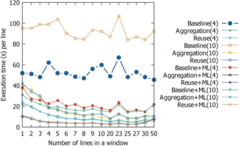
The size of the tumbling window is critical for efficient PDF computation. When it is too small, the degree of parallel execution among multiple cluster nodes is low. Increasing the window size increases the degree of parallelism, but may introduce some overhead in terms of data transfers among nodes or management of concurrent tasks. Thus, it is important to find an optimal window size in order to make a good trade-off between the degree of parallelism and overhead.
To find the optimal window size, we distinguish between the data loading process and the PDF computation process, which have different data access patterns. In data loading, the processing of each point can be done independently by a Map operation in parallel. Thus, the overhead of data transfers and concurrent task management with a big window size is small. Thus, we can choose a window size that ensures that there is enough work to do for each node and that multiple nodes can be used. For instance, consider a cluster withnnodes, each node withcCPU cores. Assuming that the data loading for each point can occupy a CPU core, we can choose a
maximum window size corresponding ton*c points. If the number of points is less thann*c, we choose the maximum number of points as the window size.
During PDF computation, the overhead of having a big window can be high since the pro-cessing of different points are not independent, in particular when we use data grouping. For instance, when the window size is bigger, the data of more points are present at each node. In order to group data, the data of each point need to be compared with the data of more points, which takes more time. In addition, there is much more data transferred among different nodes in the data shuffling process of data grouping. Furthermore, since the PDF computation takes much time, the management of concurrent tasks within each node also increases execution time for a big window. As a result, the overhead of having a big window becomes high for PDF computation.
To find an optimal window size, we test the Scala program on a small workload (with a small number of points) with different window sizes, and then use the optimal size for the PDF computation of all the points in the slice.
6 Methods to Compute PDFs
In this section, we present our methods to compute PDFs efficiently. First, we introduce a baseline method, which will be useful for comparison. Then, we propose two methods,i.e.data grouping and ML prediction, to compute PDFs, which addresses the main problem defined in Section 4. Finally, we propose a sampling method to calculate the features of a slice, which addresses the related problem.
6.1Baseline Method
The baseline method computes the PDF of each point in a slice as follows (see Algorithm 1). Line 2 loads the spatial datasets and calculates the mean and standard deviation values of each point by using Algorithm 2. Lines 3 - 13 compute the PDF for all the points in theith slice. Line 5 gets a window in the slice. Line 6 selects all the points in the window to process. The implementation of the select function is different for data grouping (see details in Section 6.2). For each point in the window, Line 8 gets the set of corresponding observation values, which can be automatically
realized by Spark as the RawData is stored in RDD with the id of a point as key and the
set of observation values as value. Line 9 computes the PDF based on the observation values and the error between the PDF and the observation values. This can be achieved by executing an R program. The loop of Lines 8-10 can be executed in parallel using the Map operation in Spark. The ComputeP DF&Error function is realized by Algorithm 3. The data is persisted in the storage resources (Line 12) and the average error E is calculated (Line 15). Lines 3-15 correspond to the PDF computation process.
Algorithm 2 loads and preprocesses the spatial data. Line 4 chooses a window to load the data. Then, for each point in the window, the data in each dataset of DS is loaded (Lines 6-10). This process is realized in a Map function in Spark. A Java program is called in the Map function to read the data at a specific position instead of loading all the data. Then, the mean and standard deviation values are calculated (Lines 11 and 12). Finally, the loaded data is cached in memory in a Spark RDD (Line 16).
Algorithm 3 computes the PDF of a point with the smallest error in a set of candidate distri-bution types. Line 3 calculates the statistical parameters of PDFs based on different distridistri-bution types in a set of distribution candidatesT ypes. For instance, the parameters for Normal are mean and standard deviation values while the parameter for exponential is rate. The more types are
Algorithm 1 PDF computation
Input: DS: a set of spatial datasets corresponding to a spatial cube area;i: theith slice to analyze;T ypes: a set of distribution types
Output: P DF: the PDF of all the points in theith slice of the cube area;E: the average error between the PDF and the observation values of all the points in theith slice
1: P DF← ∅
2: RawData←loadData(DS, i)
3: whilenot all points insliceiare processeddo
4: pdf s← ∅
5: window←GetN extW indow(slicei)
6: P oints←Select(window, RawData) 7: for eachp∈P ointsdo
8: d←getObservationV alues(p, RawData) 9: (pdf, error)←ComputeP DF&Error(d, T ypes) 10: pdf s←pdf∪pdf s
11: end for 12: persist(pdf s) 13: P DF←P DF∪pdf s 14: end while
15: E←Average(error) end
Algorithm 2 Data loading (loadData)
Input: DS: a set of datasets corresponding to a spatial cube area;i: theith slice to analyze
Output: RawData: mean, standard deviation and the original dataset of each point in the cube area 1: RawData← ∅
2: whileRawDatadoes not contain all the points insliceido
3: windowData← ∅
4: window←GetN extW indow(slicei)
5: for eachp∈windowdo 6: rd← ∅
7: for eachds∈DSdo 8: data←GetData(ds, p, i) 9: rd←data∪rd
10: end for
11: µ←ComputeM ean(rd) 12: σ←ComputeStd(rd) 13: rd←µ∪σ∪rd
14: windowData←rd∪windowData 15: end for
16: Cache(windowData)
17: RawData←windowData∪RawData 18: end while
end
considered in T ypes, the longer the execution time of Algorithm 3 is. Then, the corresponding error of the PDF based on type and parameters are calculated using Equation 5. Finally, the PDF that incurs the smallest error is chosen (Line 7).
We exploit Algorithms 1 and 2 in both the data grouping and ML prediction methods. However, theSelectandComputeP DF&Error functions are different in different methods.
6.2Data Grouping
As some positions in the cube area may share the same physical properties, the corresponding points may have the same distribution of observation values. Thus, using the data grouping
Algorithm 3PDF computing (ComputePDF&Error)
Input: d: a set of observation values for a point;T ypes: a set of distribution types
Output: P DF: the PDF of the point;error: the error between the PDF defined by the distribution type and the statistical parameters and the observation values of the point
1: results← ∅
2: for eachtype∈T ypesdo
3: parameters←f itDistribution(d, type) .fitDistribution implemented by MLE or NM 4: pError←CalculateError(type, parameters, d) .According to Equation 5 5: results← {(type, parameter, pError)} ∪results
6: end for
7: (P DF, error)←GetSmallestError(results) end
method, we can execute the PDF computation process only once and use the result to represent all the corresponding points. In this method, theSelectfunction in Algorithm 1 has two steps. First, the points with exactly the same mean and standard deviation values are aggregated into a group. The grouping can be realized by theaggregation operation in Spark. Then, one point in each group is selected to represent the group of points. Then, the data corresponding to selected points are processed to compute the PDFs.
We randomly select one point in an aggregated group. We assume that the points that share the same mean and standard deviation have the same PDF although their observation values can be different. With this assumption, the selection of the point in an aggregated group does not have an effect on the computed PDF of the group. There are scenarios where the mean and standard deviations share the same values, respectively, but the PDFs are different. In this situation, we can take into consideration other normalized moments1,e.g.3rd, 4th etc. However, it may take additional time to calculate other normalized moments. Thus, we only consider the mean and standard deviations. We will experiment with datasets where the points of the same set of mean and standard deviation values have the same PDFs.
In some cases, although some points may share the same PDF, the observation values of the points are slightly different. And the mean and standard values may be different by a very small fluctuation. In this case, we can cluster the points that have similar mean and standard deviation values with an acceptable error. For instance, we can use k-means [33], which is already implemented in parallel within Spark MLlib. However, the implementation of point clustering is out of the scope of this paper and we leave it as future work.
When the number of nodes in the cluster is small and the window size is small, there is few data to be transferred for the grouping. And the grouping method can avoid repeated execution on the same set of observation values. However, when the number of nodes is high or the window size is big, there is much more data to be transferred among different nodes, which may take much time. In some situations, the time to transfer the data may be longer than the time to run the repeated execution. In addition, if a point corresponds to big amounts of data (many observation values), even though the window size is small, the shuffling process of data grouping may also take much time. In this case, the data grouping method is not efficient.
1Thenth moment is defined as:
µn= m
X
i=1
(xi−µ)n (7)
wheremis the number of values in the dataset,xiis theith value in the dataset andµis the mean value of the
Fig. 7: A decision tree to choose the distribution type for a set of data.
6.2.1Reuse Optimization
When there are points of the same mean and standard deviation values in different windows, we can reuse the existing calculated results in order to avoid new executions. Thus, we propose the reuse optimization method, which not only aggregates the data to groups but also checks if there are already existing results,i.e.the PDFs for the point of the same mean and standard deviation values, generated from the previous execution of processed windows. We expect this method to be better than data grouping only. However, it may take time to store all the calculated results and to search existing PDFs from a large list of previously generated results. This extra time
may be longer than the reduced time, i.e. the time to compute the PDF on the dataset (the
execution time of Algorithm 3).
6.3ML Prediction
In this section, we propose an ML prediction method based on a decision tree to compute PDFs. Decision tree classifier [38] is a typical ML technique to classify an object into different categories. The basic idea is to break up a complex decision into a union of several simpler decisions, hoping the final solution obtained this way would resemble the intended desired solution. The decision tree can be described as a tree selected from a lattice [7]. A treeG= (V, E) consists of a finite, nonempty set of nodesV and a set of edgesE. A path in a tree is a sequence of edges. The depth of the graph in a tree is the length of the largest path from the root to a leaf. A leaf is the node that has no proper descendant.
The data to be used to generate a decision tree is training data. In order to generate a decision tree, the training data can be split into different datasets (bins) according to different features and each dataset is a unit to be processed. The maximum number of bins is defined in order to reduce the time to generate a decision tree. Figure 7 shows a decision tree of depth 3 to choose a distribution type for a dataset. However, in this paper, we take some statistical features as parameters to choose a distribution as explained below.
In Algorithm 3, the execution of Lines 3-5 is repeated several times (the number of distribution type candidates), which is very inefficient. We assume that we can learn the correlation among
statistical features,e.g. mean and standard deviation values, and the distribution type. Then, we can directly predict the distribution type based on the relationship and use the predicted distribution type to execute Lines 3-5 in Algorithm 3 once for each point.
We assume that we have some previously generated output data, which contains the results of several points, i.e. the mean and standard deviation values and the type of distribution. Before execution of our method, we can generate a ML model (that correlates between statistical features and distribution types),i.e.decision tree, based on the previous existing data. Then, we use Algorithm 4 to replace Algorithm 3.
When the points in the current slice have the same correlation between the statistical features and the distribution types as that in the previously generated output data, we can use ML prediction. Generally, the points in different slices but corresponding to the same spatial dataset have the same correlation. Thus, we can use the output data generated based on some points in one slice,e.g. Slice 0, to generate decision tree model and use the model to calculate PDFs of the points in other slices,e.g.Slice 201. This correlation information is not based on the fact that various points present the same statistical features,e.g.PDF, although this fact is general since the positions in the cube area related to the points may share similar physical properties. The correlation is related to each set of datasets and corresponds to a cube area. In addition, we can find that the correlation information in Slice 0 can always be used in our targeted slice with a few acceptable extra errors as shown in Section 7.
Algorithm 4PDF computing based on ML prediction
Input: d: a vector of observation values for a point; model: the decision tree; µ: the mean value of d;σ: the standard deviation value ofd
Output: T: the distribution type of the point;P: the parameters of the distribution;error: the error between the PDF defined by the distribution type and the parameters of the distribution and the real distribution of data ind
1: T ←predict(model, µ, σ) 2: P ←f itDistribution(d, T)
3: error←CalculateError(T , P, d) .According to Equation 5
end
6.3.1ML Model Generation
In order to generate the decision tree model, there are some hyperparameters to determine,e.g. the depth of the tree (depth) and the maximum number of bins (maxBins). In order to tune the hyperparameters, we randomly split the previously generated output data into two datasets, i.e. training set and validation set. We use the training set to train the model with different combinations of hyperparameters. Then, we test the generated models on the validation set in order to choose an optimal combination of hyperparameters. We take the wrong prediction rate in the validation set as the model error while tuning the hyperparameters. The model error represents the preciseness of the decision tree model.
The model error decreases at the beginning and then increases, because of overfitting [48], as the values ofdepth and maxBins increase. While the time to train the model becomes longer
when the values ofdepth andmaxBins increase. We choose the minimum values ofdepth and
maxBins, from which the error does not decrease when they (depthormaxBin) increase. The process to tune the hyperparameters can take much time. We assume that the points in different slices have the same correlation between the statistical features and distribution types. We also assume that the hyperparameters can be shared to train the models based on different previously
generated output data in order to avoid tuning the hyperparameters and to reduce the time to train the decision tree model. Thus, the chosen values ofdepth andmaxBinsare used as fixed hyperparameters to generate the decision tree model for different previously generated output data.
Within the previously generated output data, each point has mean and standard deviation values and the distribution type. Since we have fixed hyperparameters, we do not need to use a validation dataset to tune the hyperparameters. Thus, in order to generate the model, we randomly partition the previously generated output dataset into two parts,i.e.training set and test set. In the training processing, we train the model using the training set. The input of the trained model is the mean and standard values and the output is a predicted distribution type. After generating the model, we take the wrong prediction rate in the test set as the model error while training models. During the PDF computation process, the generated model is broadcast to all the nodes, which reduces communication cost.
There are scenarios in which the mean and standard deviation share the same values, re-spectively, but the distribution type is different. In this situation, we can take into consideration other normalized moments as explained in Section 6.2. We will experiment with datasets where the points of the same set of mean and standard deviation values have the same distribution types.
6.4Complexity Analysis
Since the ML approach optimizes theComputeP DF&Error function, it can be combined with other methods as shown in Table 1. Thus, we call the pure adoption of ML: ML or baseline + ML; the combination of data grouping and ML: data grouping + ML or grouping + ML; the combination of reuse and ML: reuse + ML. Grouping + ML first uses the data grouping methods to group points and then use ML prediction to calculate PDF and error for each representative point. Reuse + ML first groups the points using the data grouping method and then searches the PDF corresponding to the set of the mean and standard deviation values of each representative point in the results generated by previous execution. If there is no results for the set of mean and standard deviation values, it uses the ML method to calculate the PDF and the error.
Name Configuration Select Function in Algorithm 1 Algorithms Reuse Baseline No data grouping or ML Select all the points 1, 3 No Grouping Data grouping without ML Select one point per group 1, 3 No Reuse Reuse without ML Select one point per group 1, 3 Yes
ML Baseline with ML Select all the points 1, 4 No
Grouping + ML Data grouping with ML Select one point per group 1, 4 No Reuse + ML Reuse with ML Select one point per group 1, 4 Yes
Table 1: Configuration of different methods. Reuse represents that the process tries to
reuse the calculated PDFs corresponding to the same mean and standard deviation values in other windows (see details in Section 6.2.1).
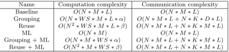
Table 2 shows the computation complexity and the communication complexity of different combinations of methods. Letα(the same as that in Table 2) represent the average ratio between the number of points that have different sets of mean and standard values and the total number of points in a window. β (the same as that in Table 2) represents the average ratio between the number of points that have different sets of mean and standard values and the number of all points in a slice. The “average” inαandβis calculated in terms of the whole data set. Thus,βis smaller
thanαwhen there are points that have the same set of mean and standard deviation values1.
W S represents the window size. When W S∗αis bigger than 1, the computation complexity
of Grouping is bigger than Baseline. In this case, we ignore data grouping. When N∗W S∗β is bigger than 1, the computation complexity of Reuse is bigger than that of Baseline. When N increases, the computation complexity of Reuse increases much faster than Baseline because ofN2. The communication complexity of Grouping and Reuse is bigger than that of Baseline. When the number of nodes in a cluster g or the number of observation values for each point get big, the communication complexity of Grouping or Reuse increases linearly, which corresponds to longer execution time. When combining with ML, Grouping and Reuse have the same features, i.e.bigger computation complexity whenW S∗α(N∗W S∗β for Reuse) is bigger than 1 and bigger communication complexity. The computation complexity of ML is smaller than that of Baseline, which corresponds to smaller execution time as shown in Section 7. In addition, ML has the same communication complexity as that of Baseline.
Name Computation complexity Communication complexity
Baseline O(N∗M∗L) O(N∗M∗L)
Grouping O(N∗W S∗M∗L∗α) O(N∗M∗L+N∗K∗D∗L) Reuse O(N2∗W S∗M∗L∗β) O(N∗M∗L+N∗K∗M∗L)
ML O(N∗M) O(N∗M∗L)
Grouping + ML O(N∗M∗W S∗α) O(N∗M∗L+N∗K∗M∗L) Reuse + ML O(N2∗M∗W S∗β) O(N∗M∗L+N∗K∗M∗L)
Table 2:Computation and communication complexity of different methods. N
repre-sents the number of points.M represents the number of observation values for each point. L represents the number of distribution types in Algorithm 3. W S represents the window size. K represents the number of nodes in a cluster. αrepresents the ratio between the number of points that have different sets of mean and standard values and the total number of points in a window.β represents the ratio between the number of points that have different sets of mean and standard values and the number of all the points in a slice.
6.5Sampling
In order to choose a slice to compute PDFs, we need to compute the features of a slice very quickly. We propose a sampling method (see Algorithm 5) that samples the points and uses ML prediction to generate the distribution type of each point. This method does not run the statistical calculation of the each point in theComputeP DF&Errorfunction in Algorithm 1 in order to reduce execution time.
In Algorithm 5, Line 1 samples the points in slicei based on a predefined sampling rate. A sampling rate represents the ratio between the selected points from the sampling process and all the original points. Lines 3-13 implement the process that loads the data from the datasets and calculates the mean and standard deviation values for each double sampled point. Line 14 groups the data as explained in Section 6.2. When the number of nodes in the cluster is high, we can
1Letn
window be the number of points that have different sets of mean and standard values in a window and
Nwindow be the total number of points in a window. Then,α= Nnwindow
window. We assume that there arelwindows in a slice. When the points in different windows have different sets of mean and standard deviation values,β=
l∗nwindow
l∗Nwindow =α. Whenkpoints have same sets of mean and standard deviation values in two different slices,β= l∗nwindow−k
remove Line 14 in order to reduce the time of shuffling. Lines 16 - 19 calculate the distribution type of each double sampled point based on a decision tree (see Section 6.3.1 for details). Lines 21 - 25 calculate the final results,i.e.the average mean value, the average standard deviation and the percentage of different distribution types. Lines 16 - 25 correspond to the PDF computation process.
Algorithm 5 Sampling process
Input: DS: a set of datasets produced by simulations; i: the ith slice to analyze; model: the decision tree corresponding to the relationship between the mean and standard value and the distribution type;T ypes: a set of distribution types;rate: the sampling rate
Output: µ: the average mean value of the slice;σ: the average standard deviation of the slice;T ypesP ercentage: the percentage of distribution types of the points in the slice
1: P oints←Sample(slicei, rate)
2: RawData← ∅ 3: for eachp∈pointsdo 4: rd← ∅
5: for eachds∈DSdo 6: data←GetData(ds, p, i) 7: rd←data∪rd
8: end for
9: µ←ComputeM ean(rd) 10: σ←ComputeStd(rd) 11: rd←µ∪σ∪rd
12: RawData←rd∪RawData 13: end for
14: P oints←selectByGrouping(RawData) 15: allT ypes← ∅
16: for eachp∈P ointsdo
17: type←predict(model, RawData) 18: allT ypes←type∪allT ypes 19: end for
20: T ypesP ercentage← ∅ 21: for eachtype∈T ypesdo
22: pct←calculateP ercentage(type, allT ypes) 23: T ypesP ercentage←pct∪T ypesP ercentage 24: end for
25: (µ, σ)←averageCalculation(RawData) end
We can randomly sample the points. The random sampling method takes much time while the selected points may contain little repeated information. We could also use a k-means clustering algorithm [33] and choose the point that is the closest to the center of each cluster as double sampled points. The double sampled data generated by k-means contains diverse information, which does not help much to choose a slice (see details in Section 7.2.3). Furthermore, k-means may take much time to converge. Therefore, instead of k-means, we use random sampling in Algorithm 5.
7 Experimental Evaluation
In this section, we evaluate and compare the different methods presented in Section 6 for different datasets and cluster sizes. To ease reading, we call each method by a name as: Baseline, Grouping, Reuse, ML and Sampling. First, we introduce the experimental setup, with two different clusters
(a small one and a big one). Then, we perform experiments with a 235 GB dataset. Finally, we perform experiments with big datasets (1.9 TB and 2.4 TB).
7.1Experimental Setup
In this section, we present the different spatial datasets, the candidate distribution types (see Algorithms 3 and 5) and the cluster testbeds, which we use in our various experiments.
To generate the spatial data, we use the UQlab framework [32] to produce 16 values as the input parameters,i.e.V p, of the models from the seismic benchmark of the HPC4e project [2]. The input parameters obey four distribution types,i.e. normal, exponential, uniform and log-normal. In each simulation, we generate a set of the input parameters according to the PDF of each layer and generate a spatial dataset by using the set of the input parameters and the models. We run the simulation multiple times and generate three sets of spatial datasets, denoted bySet1, Set2 andSet3. The simulation is repeated 1000 times to generateSet1.Set1 contains 1000 files, each of which is a spatial dataset and has 235 GB. InSet1, the dimension of the cube area is 251 * 501 * 501,i.e.501 slices, each slice has 501 lines and each line is composed of 251 points. To generateSet2, we run the simulation 1000 times while the dimension is 501 * 1001 * 1001.Set2 has 1.9 TB. A point is associated to 1000 observation values in bothSet1 andSet2. Finally, we run the simulation 10000 times with the dimension of 251 * 501 * 501 in order to generateSet3, which has 2.4 TB. In this dataset, a point is associated to 10000 observation values. We use the same slice (Slice 201 because it has interesting information) in all the experiments. We consider two sets of candidate distribution typesT ypes, introduced in Algorithms 3 and 5. The first set is the set of distribution types of the input parameters, i.e. normal, exponential, uniform and log-normal, since we assume that the distribution types of different points are within those of the input parameters of the simulation. In addition, we assume that the distribution types may belong to other types beyond the scope of the distribution types of the input parameters because of non-linear relationship between the input parameters and the values of each point of the spatial cube area. With this assumption, we have a second type of candidate distribution types, i.e.normal, exponential, uniform, log-normal, Cauchy, gamma, geometric, logistic, Student’s t and Weibull. We call the first set 4−typesand the second 10−types.
We use two cluster testbeds, each with NFS, HDFS and Spark deployed. The first one, which we call LNCC cluster, is a cluster located at LNCC with 6 nodes, each having 32 CPU cores and 94 GB memory. The second one is a cluster of Grid5000, which we call G5k cluster, with 64 nodes, each having 16 CPU cores and 131 GB of RAM storage.
7.2Experiments on a 235 GB Dataset
In this section, we compare the different methods based on the spatial dataset Set1 of 235 GB. First, we compare the performance of different methods using the LNCC cluster: Baseline, Grouping, Reuse and the combination of these methods with ML. Then, we study the scalability of different methods using the G5k cluster. Finally, we study the performance of Sampling.
We take the relationship between the set of mean and standard deviation values and the distribution types of 25000 points in Slice 0 in the previously generated output data of Set1 to tune the hyperparameters of the decision tree. The hyperparameters are tuned at the very beginning, which takes 18 minutes for 4−typesand 22 minutes for 10−typesusing Spark on a workstation with 8 CPU cores and 32 GB of RAM.
We take advantage of the previously generated output data ofSet1 to generate the decision tree model for the experiments of this section. The model error is 0.03 for 4−types, and 0.08 for
0 100 200 300 400 500 600
Baseline Grouping Reuse
4-types + Baseline 10-types + Baseline 4-types + ML 10-types + ML
Fig. 8: Execution time for PDF computation on a small workload (6 lines and 3006
points) with 235 GB input data.The time unit is second.
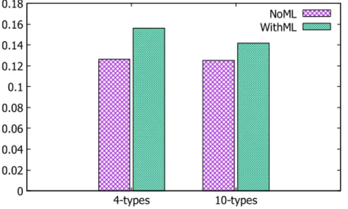
0 0.02 0.04 0.06 0.08 0.1 0.12 0.14 0.16 0.18
4-types 10-types
NoML WithML
Fig. 9:Error in PDF computation.NoML represents the error of different methods without
adoption of ML,i.e.Baseline, Grouping and Reuse with 4−typesor 10−types(see Figure 8).
WithML represents the combinations of methods with ML,i.e.Baseline + ML, Grouping + ML,
Reuse + ML with 4−typesor 10−types(see Figure 8).
10−types. Although the model error of 10−typesis bigger than that of 4−types, the average error E in Algorithm 1 is smaller. The time to train the model ranges from 1 to 20 seconds, which is negligible compared with the execution time of the whole PDF computation process. 7.2.1Performance Comparisons
In this section, we compare the performance of different methods,i.e.Baseline, Grouping, Reuse, and the combination with ML, using the LNCC cluster. First, we execute the Scala program (for computing PDFs with different methods) on a small workload (6 lines and 3006 points). Second, we compare the performance of different methods for different window sizes. Finally, we compare the performance of different methods with the tuned window size for the whole slice.
Experiments with Small Workload In this section, we use a small workload of 6 lines,i.e.3006 points, to compare the performance of different methods. The execution time for PDF compu-tation is shown in Figure 8 and the error is shown in Figure 9.