Model-Driven One-Sided Factorizations on Multicore
Accelerated Systems
Jack Dongarra1 2 3, Azzam Haidar1, Jakub Kurzak1, Piotr Luszczek1,
Stanimire Tomov1, Asim YarKhan1
Hardware heterogeneity of the HPC platforms is no longer considered unusual but instead have become the most viable way forward towards Exascale. In fact, the multitude of the hetero-geneous resources available to modern computers are designed for different workloads and their efficient use is closely aligned with the specialized role envisaged by their design. Commonly in order to efficiently use such GPU resources, the workload in question must have a much greater degree of parallelism than workloads often associated with multicore processors (CPUs). Available GPU variants differ in their internal architecture and, as a result, are capable of handling work-loads of varying degrees of complexity and a range of computational patterns. This vast array of applicable workloads will likely lead to an ever accelerated mixing of multicore-CPUs and GPUs in multi-user environments with the ultimate goal of offering adequate computing facilities for a wide range of scientific and technical workloads. In the following paper, we present a research prototype that uses a lightweight runtime environment to manage the resource-specific workloads, and to control the dataflow and parallel execution in hybrid systems. Our lightweight runtime environment uses task superscalar concepts to enable the developer to write serial code while pro-viding parallel execution. This concept is reminiscent of dataflow and systolic architectures in its conceptualization of a workload as a set of side-effect-free tasks that pass data items whenever the associated work assignment have been completed. Additionally, our task abstractions and their parametrization enable uniformity in the algorithmic development across all the heterogeneous resources without sacrificing precious compute cycles. We include performance results for dense linear algebra functions which demonstrate the practicality and effectiveness of our approach that is aptly capable of full utilization of a wide range of accelerator hardware.
Keywords: hardware accelerators, dense linear algebra, task superscalar scheduling.
1. Introduction
With the release of CUDA in 2007, the communities of scientific, HPC, and technical com-puting started to enjoy the performance benefits of GPUs. The ever expanding capabilities of the hardware accelerators allowed GPUs to deal with more demanding kinds of workloads and there was very little need to mix different GPUs in the same machine. Intel offering in the realm of hardware acceleration came in the form of a coprocessor called MIC (Many Integrated Cores) now known as Xeon Phi and available under Knights Corner moniker. In terms of capabilities, on the one hand, they are similar to those of GPUs but, on the other hand, there are some slight differences in workloads that could be handled by Phi. We do not intend in this paper to com-pare between GPUs and the recently introduced MIC coprocessor. Instead, we take a different stand because we believe that the users will combine CPUs, GPUs, and coprocessors to leverage strengths of each of them depending on the workload. In a similar fashion, we are showing here how to combine their strengths to arrive at another level of heterogeneity by simultaneously utilizing all three: CPUs, GPUs, and coprocessors. We call this a multi-way heterogeneity for which we present a unified programming model that alleviates the complexity of dealing with multiple software stacks for computing, communication, and software libraries.
1University of Tennessee, Knoxville, USA
2. Background and Related Work
This paper presents research in algorithms and a programing model for high-performance dense linear algebra (DLA) factorizations for heterogeneous multiple multicore CPUs, GPUs, and Intel Xeon Phi coprocessors (MICs). The mix can contain resources with varying capabilities, e.g., CUDA GPUs same architecture but from different device generations. While the main goal is to obtain as high fraction of the peak performance as possible for an entire heterogeneous system, an often competing secondary goal is to propose a programming model that would simplify the development. To this end, we propose and develop a new lightweight runtime environment, and a number of dense linear algebra routines based on it. We demonstrate the new algorithms, their performance, and the programming model design using the Cholesky and QR factorizations.
2.1. High Performance on Heterogeneous Systems
Efficient use of current computer architectures, namely, running close to their peak per-formance, can only be achieved for algorithms of high computational intensity. In the specific context of DLA, O(n2) data requires O(n3) floating point operations (flop’s). In contrast, less compute intensive algorithms that use sparse linear algebra can reach only a fraction of the peak performance, e.g., a few Gflop/s for highly optimized sparse matrix-vector multiply (SpMV) [6] versus over 1000 Gflop/s for double-precision matrix-matrix multiply (DGEMM) on a Kepler K20c GPU [11]. This highlights the interest in DLA and the importance of designing computa-tional applications that can make efficient use of the available hardware resources.
Early results for DLA were tied to development of high performance Basic Linear Algebra Subroutines (BLAS). Volkov el al. [30] developed fast single-precision matrix-matrix multiply (SGEMM) for the NVIDIA Tesla GPUs and highly efficient LU, QR, and Cholesky factorizations based on that. The fastest DGEMM and factorizations based on it for the NVIDIA Fermi GPUs were developed by Nath et al. [20]. These early BLAS developments were eventually incorporated into the CUBLAS library [11]. The main DLA algorithms from LAPACK were developed for a single GPU and released through the MAGMA library [19].
More recent work has concentrated on porting additional algorithms to GPUs, and on various optimizations and algorithmic improvements. The central challenge has been to split the computation among the hardware components to efficiently use them, to maintain balanced load, and to reduce idle times. Although there have been developments for a particular accelerator and its multicore host [3, 5, 9, 12, 25, 26], to the best of our knowledge there has been no efforts to create a DLA library on top of a unified framework for multi-way heterogeneous systems.
2.2. Heterogeneous parallel programming models
Task superscalar runtime environments have become a common approach for effective and efficient execution in multicore environments. This task scheduling mechanism has its roots in dataflow execution, which has a long history dating to the nineteen sixties [7, 16, 24]. It has seen a reemergence in popularity with the advent of multicore processors in order to use the available resources dynamically and efficiently. Many other programming methodologies need to be carefully managed in order to avoid fork-join style parallelism, also called Bulk Synchronous Processing [29], which is increasingly wasteful in face of ever larger numbers of cores in a single CPU socket.
In our current research, we build on the QUARK [31, 32] runtime environment to demon-strate the effectiveness of dynamic task superscalar execution in the presence of heterogeneous architectures. QUARK is a superscalar execution environment that has been used with great success for linear algebra software on multicore platforms. The PLASMA linear algebra library has been implemented using QUARK and has demonstrated excellent scalability and high per-formance [2, 17].
There is a rich area of work on execution environments that begin with serial code and result in parallel execution, often using task superscalar techniques, for example Jade [23], Cilk [8], Sequoia [13], SuperMatrix [10], OmpSS [22], Habanero [5], StarPU [4], or the DepSpawn [14] project.
We chose QUARK as our lightweight runtime environment for this research because it provides flexibility in low level control of task location and binding that would be harder to obtain using other superscalar runtime environments. But, the conceptual work done in this research could be replicated within other projects, so we view QUARK simply as a convenient representative of a lightweight, task-superscalar runtime environment.
Both GPUs and Intel Xeon Phi coprocessors provide high degree of parallelism that can deliver excellent application performance for DLA. However, it is important to understand the distinctions in programming models between GPUs and Intel Xeon Phi coprocessors.
2.2.1. CUDA
CUDA utilizes a large number of concurrent threads of execution to exploit hardware par-allelism and achieve high performance. CUDA threads are grouped together into blocks that execute concurrently on the GPU Streaming Multiprocessors (SMs) following the SIMD execu-tion model. NVIDIA Kepler K20 GPU has 2496 CUDA cores and delivers 1.17 Tflop/s in peak double precision floating point performance.
2.2.2. MIC Architecture and Programming Models
The Intel Xeon Phi coprocessor comprises of 61 Intel Architecture (IA) cores. Additionally, there are 8 memory controllers supporting up to 16 GDDR5 channels delivering a theoreti-cal bandwidth of 352 GB/s [1]. Its peak double precision floating point performance is 1200 Gflop/s. Unlike a GPU, the Xeon Phi coprocessor runs a Linux operating system and provides x86 compatibility. It supports popular programming models used on multi-core architectures including MPI, OpenMP and Threading Building Blocks. Xeon Phi also offers the following flexible programming models depending on applications:
• Native model: It is used to run applications entirely on a Xeon Phi coprocessor like any
• Offload model: It is used to utilize a Xeon Phi coprocessor as an accelerator to execute computation intensive regions of an application offloaded from host.
Offloading incurs overhead costs for initialization, marshaling and transferring data, and code invocation. Applications must have a high ratio of computation to communication for the offloaded portion. Offload communication overheads can be hidden if code is structured to overlap them with computation, or if data is reused across offload regions [21]. To effectively make use of this model, asynchronous offload features must be used, which include: asynchronous data transfer, asynchronous compute and memory management without data transfer. Signal and wait clauses need to be used in offload pragmas and directives to enable asynchronous data transfer and computation. For example:
offload transfer pragma/directive called with a signal clause begins an asynchronous data
transfer.
offload pragma/directive called with a signal clause begins an asynchronous computation.
offload wait pragma/directive called with a wait clause blocks execution until an asynchronous
data transfer or computation is complete.
At this point, this programming model has been codified by the OpenMP 4.0 standard and may be considered analogous to the OpenACC standard initially implemented on GPUs only.
Beside the above programming models, Intel provides two software libraris – SCIF (Sym-metric Communication Interface) and COI (Coprocessor Offload Infrastructure) – to ease the development of software tools and applications that run on the Xeon Phi Coprocessor.
• SCIF (Symmetric Communication Interface) is an API for communication between pro-cesses on MIC and the host CPU within the same system. It resembles POSIX socket inter-face whereby connections are established usingscif listen,scif connect, andscif accept rou-tines. For efficient communication between the processes SCIF API provides send-receive semantics where one serves as the source and the other as the destination of the com-munication channel. Efficient data transfer is ensured by Remote Memory Access (RMA) semantics where a region of memory needs to be registered (using scif register first and scif unregister afterwards) for remote access. Upon registration, further data transfers (us-ing scif readfrom and scif writeto can occur in a one-sided manner with just one process either reading from or writing to a memory window. These reads and writes can make both synchronous and asynchronous progress and the completion of asynchronous RMA operations is checked usingscif fence mark and scif fence wait routines.
• COI (Coprocessor Offload Infrastructure) model exposes a pipelined programming model to the user. This model allows workloads to run and data to be moved asynchronously, allowing the host processor, device processor, and DMA engines to remain busy simultane-ously and independently. This library provides services to create coprocessor-side processes, create FIFO pipelines between the host and coprocessor, move code and data, invoke code (functions) on the coprocessor, manage memory buffers that span the host and coprocessor, enumerate available resources, and so on [21].
3. BLAS
1 f o r (m = 0 ; m<M; m++) 2 f o r ( n = 0 ; n<N ; n++) 3 f o r ( k = 0 ; k<K ; k++) 4 C [ n ] [ m] += A [ k ] [ m]∗B [ n ] [ k ] ;
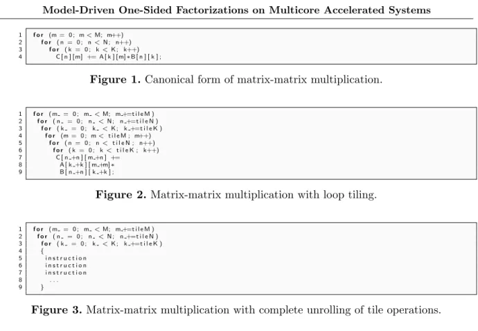
Figure 1.Canonical form of matrix-matrix multiplication.
1 f o r ( m = 0 ; m <M; m +=t i l e M ) 2 f o r ( n = 0 ; n <N ; n +=t i l e N ) 3 f o r ( k = 0 ; k <K ; k +=t i l e K ) 4 f o r (m = 0 ; m< t i l e M ; m++) 5 f o r ( n = 0 ; n< t i l e N ; n++) 6 f o r ( k = 0 ; k< t i l e K ; k++) 7 C [ n +n ] [ m +n ] +=
8 A [ k +k ] [ m +m]∗
9 B [ n +n ] [ k +k ] ;
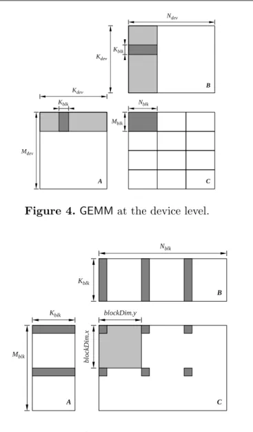
Figure 2. Matrix-matrix multiplication with loop tiling.
1 f o r ( m = 0 ; m <M; m +=t i l e M ) 2 f o r ( n = 0 ; n <N ; n +=t i l e N ) 3 f o r ( k = 0 ; k <K ; k +=t i l e K )
4 {
5 i n s t r u c t i o n 6 i n s t r u c t i o n 7 i n s t r u c t i o n 8 . . .
9 }
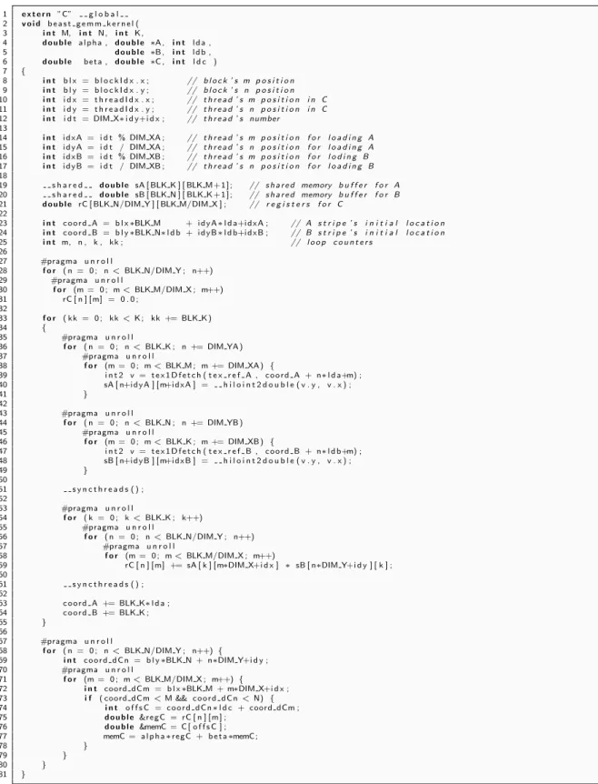
Figure 3. Matrix-matrix multiplication with complete unrolling of tile operations.
and most performance-critical BLAS routine, more so in the context of the factorizations that we consider in this paper. This section presents the process of building a fast matrix-matrix multiplication kernel for the GPU in double precision and in real arithmetic (DGEMM) by using the process of autotuning. The target is the NVIDA K40c card.
In its canonical form, matrix-matrix multiplication is represented by three nested loops as is shown in Figure 1. The primary tool in optimizing matrix-matrix multiplication is the technique of loop tiling. Tiling replaces a single loop with two loops: the inner loop that increments the iteration counter by one, and the outer loop that increments the iteration counter by the tiling factor. In the case of matrix-matrix multiplication, tiling replaces the three loops of Figure 1 with the six loops of Figure 2. Tiling of the matrix-matrix multiplication exploits thesurface to volume effect mentioned before: execution of O(n3) floating-point operations over O(n2) data.
Next, the technique of loop unrolling is applied, which replaces the three innermost loops with a single block of straight-line of code (a single basic block), as shown schematically in Figure 3. The purpose of unrolling is twofold: to reduce the penalty of looping (the overhead of incrementing loop counters, advancing data pointers and conditional branching), and to increase instruction-level parallelism by creating long sequences of independent instructions, which can fill out the processor’s pipeline and thus increase the instruction issue rate.
This optimization sequence is universal for almost any computer architecture, including “standard” superscalar processors with cache memories, as well as GPU accelerators and other less conventional architectures. Tiling, also referred to as blocking, is often applied multiple times to accommodate successive levels of cache, the registers file, TLB, etc.
Mdev
Ndev
Kdev
Kdev
Nblk Kblk
Kblk
Mblk
A
B
C
Figure 4. GEMM at the device level.
Nblk
Mblk
Kblk
Kblk blockDim.y
bl
oc
kD
im
.x
A
B
C
Figure 5.GEMM at the block level.
applied until the point where the register file is exhausted. Unrolling the inner loop beyond that point, can be used to further reduce the overhead of looping.
Figure 4 shows the GPU implementation of matrix-matrix multiplication at the device level. Each thread block computes a tile ofC(dark gray) by passing through a stripe ofAand a stripe of B (light gray). The code iterates over A and B in chunks of Kblk (dark gray). The thread
block follows the cycle of:
• making texture reads of the small, dark gray, stripes of A and B and storing them in shared memory,
• synchronizing threads with the syncthreads()call,
• loading A and B from shared memory to registers and computing the product, • synchronizing threads with the syncthreads()call.
After the complete sweep of the light gray stripes of A and B completes, the tile of C is read, updated and stored back to the device memory. Figure 5 shows closer what happens in the inner loop. The light gray area shows the shape of the thread block. The dark gray regions show how a single thread iterates over the tile.
Figure 6 shows the complete kernel implementation in CUDA. Tiling is defined by BLK M,
DIM YA define how the thread block covers a stripe of A, and finallyDIM XB and DIM YB define how the thread block covers a stripe of B.
In lines 24–28 the values of C are set to zero. In lines 32–38 a stripe of A is read (texture reads) and stored in shared memory. In lines 40–46 a stripe of B is read (texture reads) and stored in shared memory. The syncthreads()call in line 48 ensures that the process of reading ofAand B, and storing in shared memory, is finished before operation continues. In lines 50–56 the product is computed, using the values from shared memory. The syncthreads() call in line 58 ensures that computing the product is finished and the shared memory can be overwritten with new stripes of A and B. In lines 60 and 61 the pointers are advanced to the location of new stripes. When the main loop completes, C is read from device memory, modified with the accumulated product, and written back, in lines 64–77. The use of texture reads with clamping eliminates the need for cleanup code to handle matrix sizes not exactly divisible by the tiling factors.
With the parametrized code in place, what remains is the actual autotuning process, i.e., finding good values for the nine tuning parameters. Here the process used in the Bench-testing Environment for Automated Software Tuning (BEAST) project is described. It relies on three components:
1. defining the search space,
2. pruning the search space by applying filtering constraints, and
3. benchmarking the remaining configurations and selecting the best performer.
The important point in the BEAST project is to not introduce artificial and/or arbitrary limi-tations on the search process.
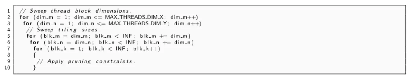
The loops in Figure 7 define the search space for the autotuning of the matrix-matrix multiplication of Figure 6. The two outer loops sweep through all possible 2D shapes of the thread block – up to the device limit in each dimension. The three inner loops sweep through all possible tiling sizes – up to arbitrarily high values, represented by the INF symbol. In practice, the actual values to substitute for the INF symbols can be found by choosing a small starting point, e.g., (64, 64, 8), and going up until further increase has no effect on the number of kernels that pass the selection process based on pruning constraints.
The list of pruning constraints consists of nine simple checks that eliminate kernels deemed inadequate for one of several reasons:
• The kernel would not compile because it exceeded a hardware limit.
• The kernel would compile but failed to launch because it exceeded a hardware limit. • The kernel would compile and launch, but produced invalid results due to the limitations
of the implementation, e.g., unimplemented corner case.
• The kernel would compile, launch, and produce correct results, but have no chance of running fast, due to an obvious performance shortcoming, such as very low occupancy. The nine checks rely on basic hardware parameters, which can be obtained by querying the card with the CUDA API. The parameters include:
1. The number of threads in the block is not divisible by the warp size. 2. The number of threads in the block exceeds the hardware maximum.
1 e x t e r n ”C” g l o b a l 2 v o i d b e a s t g e m m k e r n e l ( 3 i n t M, i n t N, i n t K ,
4 d o u b l e a l p h a , d o u b l e ∗A , i n t l d a , 5 d o u b l e ∗B , i n t l d b , 6 d o u b l e b e t a , d o u b l e ∗C , i n t l d c ) 7 {
8 i n t b l x = b l o c k I d x . x ; // b l o c k ’ s m p o s i t i o n
9 i n t b l y = b l o c k I d x . y ; // b l o c k ’ s n p o s i t i o n
10 i n t i d x = t h r e a d I d x . x ; // t h r e a d ’ s m p o s i t i o n i n C
11 i n t i d y = t h r e a d I d x . y ; // t h r e a d ’ s n p o s i t i o n i n C
12 i n t i d t = DIM X∗i d y+i d x ; // t h r e a d ’ s number
13
14 i n t i d x A = i d t % DIM XA ; // t h r e a d ’ s m p o s i t i o n f o r l o a d i n g A
15 i n t i d y A = i d t / DIM XA ; // t h r e a d ’ s n p o s i t i o n f o r l o a d i n g A
16 i n t i d x B = i d t % DIM XB ; // t h r e a d ’ s m p o s i t i o n f o r l o d i n g B
17 i n t i d y B = i d t / DIM XB ; // t h r e a d ’ s n p o s i t i o n f o r l o a d i n g B
18
19 s h a r e d d o u b l e sA [ BLK K ] [ BLK M+ 1 ] ; // s h a r e d memory b u f f e r f o r A
20 s h a r e d d o u b l e sB [ BLK N ] [ BLK K + 1 ] ; // s h a r e d memory b u f f e r f o r B
21 d o u b l e rC [ BLK N/DIM Y ] [ BLK M/DIM X ] ; // r e g i s t e r s f o r C
22
23 i n t c o o r d A = b l x∗BLK M + i d y A∗l d a+i d x A ; // A s t r i p e ’ s i n i t i a l l o c a t i o n
24 i n t c o o r d B = b l y∗BLK N∗l d b + i d y B∗l d b+i d x B ; // B s t r i p e ’ s i n i t i a l l o c a t i o n
25 i n t m, n , k , kk ; // l o o p c o u n t e r s
26
27 #pragma u n r o l l
28 f o r ( n = 0 ; n<BLK N/DIM Y ; n++) 29 #pragma u n r o l l
30 f o r (m = 0 ; m<BLK M/DIM X ; m++) 31 rC [ n ] [ m] = 0 . 0 ;
32
33 f o r ( kk = 0 ; kk<K ; kk += BLK K )
34 {
35 #pragma u n r o l l
36 f o r ( n = 0 ; n<BLK K ; n += DIM YA ) 37 #pragma u n r o l l
38 f o r (m = 0 ; m<BLK M ; m += DIM XA ) {
39 i n t 2 v = t e x 1 D f e t c h ( t e x r e f A , c o o r d A + n∗l d a+m) ; 40 sA [ n+i d y A ] [ m+i d x A ] = h i l o i n t 2 d o u b l e ( v . y , v . x ) ;
41 }
42
43 #pragma u n r o l l
44 f o r ( n = 0 ; n<BLK N ; n += DIM YB ) 45 #pragma u n r o l l
46 f o r (m = 0 ; m<BLK K ; m += DIM XB ) {
47 i n t 2 v = t e x 1 D f e t c h ( t e x r e f B , c o o r d B + n∗l d b+m) ; 48 sB [ n+i d y B ] [ m+i d x B ] = h i l o i n t 2 d o u b l e ( v . y , v . x ) ;
49 }
50
51 s y n c t h r e a d s ( ) ; 52
53 #pragma u n r o l l
54 f o r ( k = 0 ; k<BLK K ; k++) 55 #pragma u n r o l l
56 f o r ( n = 0 ; n<BLK N/DIM Y ; n++)
57 #pragma u n r o l l
58 f o r (m = 0 ; m<BLK M/DIM X ; m++)
59 rC [ n ] [ m] += sA [ k ] [ m∗DIM X+i d x ] ∗ sB [ n∗DIM Y+i d y ] [ k ] ; 60
61 s y n c t h r e a d s ( ) ; 62
63 c o o r d A += BLK K∗l d a ; 64 c o o r d B += BLK K ;
65 }
66
67 #pragma u n r o l l
68 f o r ( n = 0 ; n<BLK N/DIM Y ; n++) {
69 i n t c o o r d d C n = b l y∗BLK N + n∗DIM Y+i d y ; 70 #pragma u n r o l l
71 f o r (m = 0 ; m<BLK M/DIM X ; m++){
72 i n t coord dCm = b l x∗BLK M + m∗DIM X+i d x ; 73 i f ( coord dCm<M && c o o r d d C n<N) {
74 i n t o f f s C = c o o r d d C n∗l d c + coord dCm ; 75 d o u b l e ®C = rC [ n ] [ m ] ;
76 d o u b l e &memC = C [ o f f s C ] ; 77 memC = a l p h a∗regC + b e t a∗memC ;
78 }
79 }
80 }
81 }
1 // Sweep t h r e a d b l o c k d i m e n s i o n s .
2 f o r ( dim m = 1 ; dim m<= MAX THREADS DIM X ; dim m++) 3 f o r ( d im n = 1 ; d im n<= MAX THREADS DIM Y ; di m n++) 4 // Sweep t i l i n g s i z e s .
5 f o r ( b l k m = dim m ; b l k m<INF ; b l k m += dim m ) 6 f o r ( b l k n = d im n ; b l k n<INF ; b l k n += d im n ) 7 f o r ( b l k k = 1 ; b l k k<INF ; b l k k ++)
8 {
9 // A p p l y p r u n i n g c o n s t r a i n t s .
10 }
Figure 7.The parameter search space for the autotuning of matrix multiplication.
0 10
0 200 300 400 050 600 700 800 900
0 200 400 600 800 1000 1200 1400 1600 1800
GFLOPS
nu
m
be
r
of
k
er
ne
ls
Figure 8.Distribution of the dgemmkernels.
7. The number of load instructions, from shared memory to registers, in the innermost loop, in the PTX code, exceeds the number ofFused Multiply-Adds (FMAs).
8. Low occupancy due to high number of registers per block to store C.
9. Low occupancy due to the amount of shared memory per block to read A and B.
In order to check the last two conditions, the number of registers per block, and the amount of shared memory per block are computed. Then the maximum number of possible blocks per multiprocessor is found, which gives the maximum possible number of threads per multiproces-sor. If that number is lower than the minimum occupancy requirement, the kernel is discarded. Here the threshold is set to a fairly low number of 256 threads, which translates to minimum occupancy of 0.125 on the Nvidia K40 card, with the maximum number of 2,048 threads per multiprocessor.
This process produces 14,767 kernels, which can be benchmarked in roughly one day. 3,256 kernels fail to launch due to excessive number of registers per block. The reason is that the pruning process uses a lower estimate on the number of registers, and the compiler actually produces code requiring more registers. We could detect it in compilation and skip benchmarking of such kernels or we can run them and let then fail. For simplicity we chose the latter. We could also cap the register usage to prevent the failure to launch. However, capping register usage usually produces code of inferior performance.
In comparison, CUBLAS achieves the performance of 1,225 Gflop/s using 256 threads per multiprocessor. Although CUBLAS achieves a higher number, this example shows the effec-tiveness of the autotuning process in quickly creating well performing kernels from high level language source codes. This technique can be used to build kernels for routines not provided in vendor libraries, such as extended precision BLAS (double-double and triple-float), BLAS for oddly shaped matrices (tall and skinny), etc. Even more importantly, this technique can be used to build domain specific kernels for much broader spectrum of application areas.
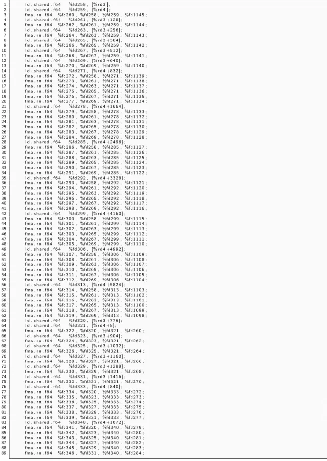
As the last interesting observation, we offer a look at the PTX code produced by NVIDIA’s
nvcc compiler (Figure 9). We can see that the compiler does exactly what is expected: it completely unrolls the loops in lines 50–56 of the C code in Figure 6 into a stream of loads from shared memory to registers followed by FMA instructions, with substantially larger number of FMAs than loads.
4. Algorithmic Advancements
In this section, we present the linear algebra aspects of our generic solution for development of either Cholesky, LU (based on Gaussian elimination), or QR (based on applying Householder reflectors) factorizations which use block outer-product updates of the trailing matrix. These three factorizations are commonly known as the one-sided factorizations because they apply a sequence of transformations on only one side of the original matrix and thus they do not preserve the matrix spectrum as thetwo-sided transformations do.
Conceptually, one-sided factorization maps a matrixAinto a product of matricesX andY:
F :
"
A11 A12 A21 A22
#
7→
"
X11 X12 X21 X22
#
×
"
Y11 Y12 Y21 Y22
#
Algorithmically, this corresponds to a sequence of in-place transformations of A, whose storage is overwritten with the entries of matricesXandY (Pij indicates the currently factorized
panels):
A(0)11 A
(0)
12 A
(0) 13
A(0)21 A
(0)
22 A
(0) 23
A(0)31 A
(0) 32 A (0) 33 →
P11 A(0)12 A
(0) 13
P21 A(0)22 A
(0) 23
P31 A(0)32 A
(0) 33 → →
XY11 Y12 Y13
X21 A(1)22 A
(1) 23
X31 A(1)32 A
(1) 33 →
XY11 Y12 Y13
X21 P22 A(1)23
X31 P32 A(1)33
→ →
XY11 Y12 Y13
X21 XY22 Y23
X31 X32 A(2)33
→
XY11 Y12 Y13
X21 X22 Y23
X31 X32 P33
→ →
XY11 Y12 Y13
X21 XY22 Y23
X31 X32 XY33
→hXYi,
whereXYij is a compact representation of bothXij and Yij in the space originally occupied by
Aij.
1 l d . s h a r e d . f 6 4 %f d 2 5 8 , [% r d 3 ] ; 2 l d . s h a r e d . f 6 4 %f d 2 5 9 , [% r d 4 ] ;
3 fma . r n . f 6 4 %f d 2 6 0 , %f d 2 5 8 , %f d 2 5 9 , %f d 1 1 4 5 ; 4 l d . s h a r e d . f 6 4 %f d 2 6 1 , [% r d 3 + 1 2 8 ] ;
5 fma . r n . f 6 4 %f d 2 6 2 , %f d 2 6 1 , %f d 2 5 9 , %f d 1 1 4 4 ; 6 l d . s h a r e d . f 6 4 %f d 2 6 3 , [% r d 3 + 2 5 6 ] ;
7 fma . r n . f 6 4 %f d 2 6 4 , %f d 2 6 3 , %f d 2 5 9 , %f d 1 1 4 3 ; 8 l d . s h a r e d . f 6 4 %f d 2 6 5 , [% r d 3 + 3 8 4 ] ;
9 fma . r n . f 6 4 %f d 2 6 6 , %f d 2 6 5 , %f d 2 5 9 , %f d 1 1 4 2 ; 10 l d . s h a r e d . f 6 4 %f d 2 6 7 , [% r d 3 + 5 1 2 ] ;
11 fma . r n . f 6 4 %f d 2 6 8 , %f d 2 6 7 , %f d 2 5 9 , %f d 1 1 4 1 ; 12 l d . s h a r e d . f 6 4 %f d 2 6 9 , [% r d 3 + 6 4 0 ] ;
13 fma . r n . f 6 4 %f d 2 7 0 , %f d 2 6 9 , %f d 2 5 9 , %f d 1 1 4 0 ; 14 l d . s h a r e d . f 6 4 %f d 2 7 1 , [% r d 4 + 8 3 2 ] ;
15 fma . r n . f 6 4 %f d 2 7 2 , %f d 2 5 8 , %f d 2 7 1 , %f d 1 1 3 9 ; 16 fma . r n . f 6 4 %f d 2 7 3 , %f d 2 6 1 , %f d 2 7 1 , %f d 1 1 3 8 ; 17 fma . r n . f 6 4 %f d 2 7 4 , %f d 2 6 3 , %f d 2 7 1 , %f d 1 1 3 7 ; 18 fma . r n . f 6 4 %f d 2 7 5 , %f d 2 6 5 , %f d 2 7 1 , %f d 1 1 3 6 ; 19 fma . r n . f 6 4 %f d 2 7 6 , %f d 2 6 7 , %f d 2 7 1 , %f d 1 1 3 5 ; 20 fma . r n . f 6 4 %f d 2 7 7 , %f d 2 6 9 , %f d 2 7 1 , %f d 1 1 3 4 ; 21 l d . s h a r e d . f 6 4 %f d 2 7 8 , [% r d 4 + 1 6 6 4 ] ; 22 fma . r n . f 6 4 %f d 2 7 9 , %f d 2 5 8 , %f d 2 7 8 , %f d 1 1 3 3 ; 23 fma . r n . f 6 4 %f d 2 8 0 , %f d 2 6 1 , %f d 2 7 8 , %f d 1 1 3 2 ; 24 fma . r n . f 6 4 %f d 2 8 1 , %f d 2 6 3 , %f d 2 7 8 , %f d 1 1 3 1 ; 25 fma . r n . f 6 4 %f d 2 8 2 , %f d 2 6 5 , %f d 2 7 8 , %f d 1 1 3 0 ; 26 fma . r n . f 6 4 %f d 2 8 3 , %f d 2 6 7 , %f d 2 7 8 , %f d 1 1 2 9 ; 27 fma . r n . f 6 4 %f d 2 8 4 , %f d 2 6 9 , %f d 2 7 8 , %f d 1 1 2 8 ; 28 l d . s h a r e d . f 6 4 %f d 2 8 5 , [% r d 4 + 2 4 9 6 ] ; 29 fma . r n . f 6 4 %f d 2 8 6 , %f d 2 5 8 , %f d 2 8 5 , %f d 1 1 2 7 ; 30 fma . r n . f 6 4 %f d 2 8 7 , %f d 2 6 1 , %f d 2 8 5 , %f d 1 1 2 6 ; 31 fma . r n . f 6 4 %f d 2 8 8 , %f d 2 6 3 , %f d 2 8 5 , %f d 1 1 2 5 ; 32 fma . r n . f 6 4 %f d 2 8 9 , %f d 2 6 5 , %f d 2 8 5 , %f d 1 1 2 4 ; 33 fma . r n . f 6 4 %f d 2 9 0 , %f d 2 6 7 , %f d 2 8 5 , %f d 1 1 2 3 ; 34 fma . r n . f 6 4 %f d 2 9 1 , %f d 2 6 9 , %f d 2 8 5 , %f d 1 1 2 2 ; 35 l d . s h a r e d . f 6 4 %f d 2 9 2 , [% r d 4 + 3 3 2 8 ] ; 36 fma . r n . f 6 4 %f d 2 9 3 , %f d 2 5 8 , %f d 2 9 2 , %f d 1 1 2 1 ; 37 fma . r n . f 6 4 %f d 2 9 4 , %f d 2 6 1 , %f d 2 9 2 , %f d 1 1 2 0 ; 38 fma . r n . f 6 4 %f d 2 9 5 , %f d 2 6 3 , %f d 2 9 2 , %f d 1 1 1 9 ; 39 fma . r n . f 6 4 %f d 2 9 6 , %f d 2 6 5 , %f d 2 9 2 , %f d 1 1 1 8 ; 40 fma . r n . f 6 4 %f d 2 9 7 , %f d 2 6 7 , %f d 2 9 2 , %f d 1 1 1 7 ; 41 fma . r n . f 6 4 %f d 2 9 8 , %f d 2 6 9 , %f d 2 9 2 , %f d 1 1 1 6 ; 42 l d . s h a r e d . f 6 4 %f d 2 9 9 , [% r d 4 + 4 1 6 0 ] ; 43 fma . r n . f 6 4 %f d 3 0 0 , %f d 2 5 8 , %f d 2 9 9 , %f d 1 1 1 5 ; 44 fma . r n . f 6 4 %f d 3 0 1 , %f d 2 6 1 , %f d 2 9 9 , %f d 1 1 1 4 ; 45 fma . r n . f 6 4 %f d 3 0 2 , %f d 2 6 3 , %f d 2 9 9 , %f d 1 1 1 3 ; 46 fma . r n . f 6 4 %f d 3 0 3 , %f d 2 6 5 , %f d 2 9 9 , %f d 1 1 1 2 ; 47 fma . r n . f 6 4 %f d 3 0 4 , %f d 2 6 7 , %f d 2 9 9 , %f d 1 1 1 1 ; 48 fma . r n . f 6 4 %f d 3 0 5 , %f d 2 6 9 , %f d 2 9 9 , %f d 1 1 1 0 ; 49 l d . s h a r e d . f 6 4 %f d 3 0 6 , [% r d 4 + 4 9 9 2 ] ; 50 fma . r n . f 6 4 %f d 3 0 7 , %f d 2 5 8 , %f d 3 0 6 , %f d 1 1 0 9 ; 51 fma . r n . f 6 4 %f d 3 0 8 , %f d 2 6 1 , %f d 3 0 6 , %f d 1 1 0 8 ; 52 fma . r n . f 6 4 %f d 3 0 9 , %f d 2 6 3 , %f d 3 0 6 , %f d 1 1 0 7 ; 53 fma . r n . f 6 4 %f d 3 1 0 , %f d 2 6 5 , %f d 3 0 6 , %f d 1 1 0 6 ; 54 fma . r n . f 6 4 %f d 3 1 1 , %f d 2 6 7 , %f d 3 0 6 , %f d 1 1 0 5 ; 55 fma . r n . f 6 4 %f d 3 1 2 , %f d 2 6 9 , %f d 3 0 6 , %f d 1 1 0 4 ; 56 l d . s h a r e d . f 6 4 %f d 3 1 3 , [% r d 4 + 5 8 2 4 ] ; 57 fma . r n . f 6 4 %f d 3 1 4 , %f d 2 5 8 , %f d 3 1 3 , %f d 1 1 0 3 ; 58 fma . r n . f 6 4 %f d 3 1 5 , %f d 2 6 1 , %f d 3 1 3 , %f d 1 1 0 2 ; 59 fma . r n . f 6 4 %f d 3 1 6 , %f d 2 6 3 , %f d 3 1 3 , %f d 1 1 0 1 ; 60 fma . r n . f 6 4 %f d 3 1 7 , %f d 2 6 5 , %f d 3 1 3 , %f d 1 1 0 0 ; 61 fma . r n . f 6 4 %f d 3 1 8 , %f d 2 6 7 , %f d 3 1 3 , %f d 1 0 9 9 ; 62 fma . r n . f 6 4 %f d 3 1 9 , %f d 2 6 9 , %f d 3 1 3 , %f d 1 0 9 8 ; 63 l d . s h a r e d . f 6 4 %f d 3 2 0 , [% r d 3 + 7 7 6 ] ;
64 l d . s h a r e d . f 6 4 %f d 3 2 1 , [% r d 4 + 8 ] ;
65 fma . r n . f 6 4 %f d 3 2 2 , %f d 3 2 0 , %f d 3 2 1 , %f d 2 6 0 ; 66 l d . s h a r e d . f 6 4 %f d 3 2 3 , [% r d 3 + 9 0 4 ] ; 67 fma . r n . f 6 4 %f d 3 2 4 , %f d 3 2 3 , %f d 3 2 1 , %f d 2 6 2 ; 68 l d . s h a r e d . f 6 4 %f d 3 2 5 , [% r d 3 + 1 0 3 2 ] ; 69 fma . r n . f 6 4 %f d 3 2 6 , %f d 3 2 5 , %f d 3 2 1 , %f d 2 6 4 ; 70 l d . s h a r e d . f 6 4 %f d 3 2 7 , [% r d 3 + 1 1 6 0 ] ; 71 fma . r n . f 6 4 %f d 3 2 8 , %f d 3 2 7 , %f d 3 2 1 , %f d 2 6 6 ; 72 l d . s h a r e d . f 6 4 %f d 3 2 9 , [% r d 3 + 1 2 8 8 ] ; 73 fma . r n . f 6 4 %f d 3 3 0 , %f d 3 2 9 , %f d 3 2 1 , %f d 2 6 8 ; 74 l d . s h a r e d . f 6 4 %f d 3 3 1 , [% r d 3 + 1 4 1 6 ] ; 75 fma . r n . f 6 4 %f d 3 3 2 , %f d 3 3 1 , %f d 3 2 1 , %f d 2 7 0 ; 76 l d . s h a r e d . f 6 4 %f d 3 3 3 , [% r d 4 + 8 4 0 ] ; 77 fma . r n . f 6 4 %f d 3 3 4 , %f d 3 2 0 , %f d 3 3 3 , %f d 2 7 2 ; 78 fma . r n . f 6 4 %f d 3 3 5 , %f d 3 2 3 , %f d 3 3 3 , %f d 2 7 3 ; 79 fma . r n . f 6 4 %f d 3 3 6 , %f d 3 2 5 , %f d 3 3 3 , %f d 2 7 4 ; 80 fma . r n . f 6 4 %f d 3 3 7 , %f d 3 2 7 , %f d 3 3 3 , %f d 2 7 5 ; 81 fma . r n . f 6 4 %f d 3 3 8 , %f d 3 2 9 , %f d 3 3 3 , %f d 2 7 6 ; 82 fma . r n . f 6 4 %f d 3 3 9 , %f d 3 3 1 , %f d 3 3 3 , %f d 2 7 7 ; 83 l d . s h a r e d . f 6 4 %f d 3 4 0 , [% r d 4 + 1 6 7 2 ] ; 84 fma . r n . f 6 4 %f d 3 4 1 , %f d 3 2 0 , %f d 3 4 0 , %f d 2 7 9 ; 85 fma . r n . f 6 4 %f d 3 4 2 , %f d 3 2 3 , %f d 3 4 0 , %f d 2 8 0 ; 86 fma . r n . f 6 4 %f d 3 4 3 , %f d 3 2 5 , %f d 3 4 0 , %f d 2 8 1 ; 87 fma . r n . f 6 4 %f d 3 4 4 , %f d 3 2 7 , %f d 3 4 0 , %f d 2 8 2 ; 88 fma . r n . f 6 4 %f d 3 4 5 , %f d 3 2 9 , %f d 3 4 0 , %f d 2 8 3 ; 89 fma . r n . f 6 4 %f d 3 4 6 , %f d 3 3 1 , %f d 3 4 0 , %f d 2 8 4 ;
Cholesky QR (Householder reflectors) LU (Gaussian Elimination)
PanelFactorize xPOTF2 xGEQF2 xGETF2 xTRSM
xSYRK2 xLARFB xLASWP
TrailingMatrixUpdate xGEMM xTRSM xGEMM
Table 1.Routines for panel factorization and the trailing matrix update.
phases leads to a straightforward iterative scheme shown in Algorithm 1. Table 1 shows BLAS and LAPACK routines that should be substituted for the generic routine names in the algorithm.
Algorithm 1:Two-phase implementation of a one-sided factorization.
forPi ∈ {P1, P2, . . . , Pn} do
PanelFactorize(Pi)
TrailingMatrixUpdate(A(i))
Algorithm 2:Two-phase implementation with a split update.
forPi ∈ {P1, P2, . . .} do
PanelFactorize(Pi)
TrailingMatrixUpdateKepler(A(i))
TrailingMatrixUpdatePhi(A(i))
The use of multiple accelerators for the computations complicates the simple loop from Algorithm 1: we have to split the update operation into multiple instances for each of the accelerators. This was done in Algorithm 2. Notice thatPanelFactorize()is not split for execution on accelerators because it is considered a latency-bound workload which faces a number of inefficiencies on throughput-oriented devices. Due to their high performance rate exhibited on the update operation, and the fact that the update requires the majority of floating-point operations, it is the trailing matrix update that should be off-loaded. The problem of keeping track of the computational activities is exacerbated by the separation between the address spaces of main memory of the CPU and the devices. This requires synchronization between memory buffers and is included in the implementation shown in Algorithm 3.
Algorithm 3: Two-phase implementation with a split update and explicit
communica-tion.
forPi ∈ {P1, P2, . . .} do
PanelFactorize(Pi)
PanelSendKepler(Pi)
TrailingMatrixUpdateKepler(A(i))
PanelSendPhi(Pi)
The code has to be modified further to achieve closer to optimal performance. In fact, the bandwidth between the CPU and the devices is orders of magnitude too slow to sustain computational rates of modern accelerators.4 The common technique to alleviate this imbalance is to use lookahead [27, 28].
Algorithm 4:Lookahead of depth 1 for the two-phase factorization.
PanelFactorize(P1)
PanelSend(P1)
TrailingMatrixUpdate{Kepler,Phi}(P1)
PanelStartReceiving(P2)
TrailingMatrixUpdate{Kepler,Phi}(R(1))
forPi ∈ {P2, P3, . . .} do
PanelReceive(Pi)
PanelFactorize(Pi)
PanelSend(Pi)
TrailingMatrixUpdate{Kepler,Phi}(Pi)
PanelStartReceiving(Pi)
TrailingMatrixUpdate{Kepler,Phi}(R(i))
PanelReceive(Pn)
PanelFactor(Pn)
Algorithm 4 shows a very simple case of lookahead of depth 1. The update operation is split into an update of the next panel, the start of the receiving of the next panel that just got updated, and an update of the rest of the trailing matrix R. The splitting is done to overlap the communication of the panel and the update operation. The complication of this approach comes from the fact that depending on the communication bandwidth and the accelerator speed, a different lookahead depth might be required for optimal overlap. In fact, the adjustment of the depth is often required throughout the factorization’s runtime to yield good performance: the updates consume progressively less time when compared to the time spent in the panel factorization.
Since the management of adaptive lookahead is tedious, it is desirable to use a dynamic Direct Acyclic Graph (DAG) scheduler to keep track of data dependences and communication events. The only issue is the homogeneity inherent in most of the schedulers which is violated here due to the use of three different computing devices that we used. Also, common scheduling techniques, such as task stealing, are not applicable here due to the disjoint address spaces and the associated large overheads of communicating the stolen task’s data across the PCI bus. These caveats are dealt with comprehensively in the remainder of the paper.
5. Lightweight Runtime for Heterogeneous Hybrid
Architectures
In this section, we discuss the techniques that we developed in order to achieve an effective and efficient use of heterogeneous hybrid architectures. What we propose, considers both the
4The bandwidth for current generation PCI Express is at most 16 GB/s and the devices achieve over 1000 Gflop/s
higher ratio of execution and the hierarchical memory model of the modern accelerators and coprocessors. Taken together, it emerges as a multi-way heterogeneous programming model. We also redesign an existing superscalar task execution environment to handle to schedule and execute tasks on multi-way heterogeneous devices.
For our experiments, we consider shared-memory multicore machines with some collection of GPUs and MIC devices. Below, we present QUARK and the specific its modifications that facilitate execution on heterogeneous devices.
5.1. Task Superscalar Scheduling
Task-superscalar execution takes as an input a sequence of tasks in a form of a DAG and schedules them for execution in parallel while honoring the data dependences between the tasks at runtime. The dependences between the tasks are honored through the resolution of data hazards: Read after Write(RaW),Write after Read(WaR) andWrite after Write(WaW). The dependences that form the DAG’s edges are extracted from the serial formulation of the code by having the user include annotations on the data items when defining the tasks. The annotations indicate whether the data is to be read and/or written.
The RaW hazard, often referred to as the true dependency, is the most common one. It defines the relation between a task writing the data and another task reading that data. The reading task has to wait until the writing task completes. In contrast, if multiple tasks wish to read the same data, they need not wait on each other but can execute in parallel once the data is available. This is the classical case of Lamport’sconcurrent events [18]. Task-superscalar execution results in an asynchronous, data-driven execution that may be represented by aDirect Acyclic Graph (DAG), where the tasks are the nodes in the graph and the edges correspond to data movement between the tasks. Task-superscalar execution is a powerful tool for productivity. Since the original code looks as if it was serial it can be written and debugged in a serial environment. After the code becomes the input for the runtime system, the parallel execution avoids all the data hazards and thus preserves the correctness of the serial code, which in turn implies the parallel correctness of execution (granted, of course, that the runtime system does not introduce conditions that violate user’s annotations).
Using task superscalar execution, the runtime can achieve parallelism by executing tasks with non-conflicting data dependences (e.g., simultaneous reads of data by multiple tasks). Superscalar execution also naturally enables lookahead into the serial code, since the tasks from the DAG representation can be executed as soon as their dependences are satisfied and not necessarily in the order they were inserted into the DAG from the the serial code.
5.2. Lightweight Runtime Environment
6. Efficient and Scalable Programming Model Across Multiple
Devices
In this section, we discuss the programming model that raises the level of abstraction above the hardware and its accompanying software stack to offer a uniform approach for algorithmic development. We describe the techniques that we developed in order to achieve an effective use of multi-way heterogeneous devices. Our proposed techniques consider both, the higher ratio of execution and the hierarchical memory model of the new emerging accelerators and coprocessors.
6.1. Supporting Heterogeneous Platforms
GPU accelerators and coprocessors have a very high computational peak compared to CPUs. For simplicity, we refer to both GPUs and coprocessors as accelerators. Also, different types of accelerators have different capabilities, which makes it challenging to develop an algorithm that can achieve high performance and exhibit good scalability. From the hardware perspective, an accelerator communicates with the CPU using I/O commands and DMA memory transfers, whereas from the software standpoint, the accelerator is a platform presented through a pro-gramming interface. The key features of our model are the processing unit capability (each of the CPUs, GPUs, Xeon Phi is assigned one such capability), the memory access overhead, and the communication cost. As with CPUs, the access time to the device memory for accelerators is slow compared to peak performance (still the accelerator memory tends to be many times faster than the CPU memory). CPUs try to improve the effect of the long memory latency and bandwidth constraint by using hierarchical caches. This does not solve the slow memory problem completely but is often effective in our target factorizations. On the other hand, accel-erators use multithreading operations that access large data sets that would overflow the size of most caches. The idea is that when the accelerator’s thread unit issues an access to the device memory, that thread unit stalls until the memory returns a value. In the meantime, the accel-erator’s scheduler switches to another hardware thread, and continues executing that thread. In this way, the accelerator exploits program parallelism to keep functional units busy while the memory fulfills the past requests. By comparison with CPUs, the device memory delivers higher absolute bandwidth (effectively around 180 GB/s for Xeon Phi and 160 GB/s for Kepler K20c). To side-step the issues related to the memory constraints, we developed a strategy that prioritizes the data-intensive operations to be executed by the accelerator and keep the memory-bound ones for the CPUs since the hierarchical caches with out-of-order superscalar scheduling are more appropriate to handle it. Moreover, in order to keep the accelerators busy, we redesign the kernels and propose dynamically guided data distribution to exploit enough parallelism to keep the accelerators and processors occupied at the same time.
Algorithm 5:Cholesky implementation for multiple devices.
Task Flags panel flags = Task Flags Initializer Task Flag Set(&panel flags, PRIORITY, 10000)
memory-bound→locked to CPU
Task Flag Set(&panel flags, BLAS2, 0)
fork∈ {0, nb,2×nb, . . . , n} do
Factorization of the panel dA(k:n,k)
Cholesky on the tile dA(k,k)
TRSM on the remaining of the panel dA(k+nb:n,k)
DO THE UPDATE: SYRK task has been split into a set of parallel compute
intensive GEMM to increase parallelism and enhance the performance. Note that
the first GEMM consists of the update of the next panel, thus the scheduler check the dependency and once finished it can start the panel factorisation of the next loop on the CPU.
if panel m>panel n then
SYRK with trailing matrix
forj∈ {k+nb, k+ 2nb, . . . , n} do
GEMM dA(j:n,k)×dA(j,k)T = dA(j:n,j)
a single source version that handles different types of accelerators either independently or when mixed together. Our intention is for our model to simplify most of the hardware details, but, at the same time, give us finer levels of control.
Algorithm 5 shows the pseudocode for the Cholesky factorization as an algorithm designer would see it. It consists of a sequential code that is simple to comprehend and independent of the architecture. Each of the calls represents a task that is inserted into the scheduler, which stores it to be executed when all of its dependencies are satisfied. Each task by itself consists of a call to a kernel function that results in execution on either a CPU or an accelerator – commonly it would called a kernel. We tried to hide the differences between hardware and let the QUARK engine handle the transfer of data automatically. In addition, we developed low-level optimizations for the accelerators, in order to accommodate hardware- and library-specific tuning and prerequisites. Moreover, we implemented a set of directives that are evaluated at runtime in order to fully map the algorithm to the hardware and to run close to the peak performance of the system. Using these strategies, we can more easily develop simple and portable code, that can run on different heterogeneous architecture and lets the scheduling and execution engine do much of the tedious bookkeeping.
In the discussion below, we will describe in detail the optimization techniques we propose, and explore some of the features of our model and also describe some directives that help with tuning performance in an easy fashion. The study here is described in the context of the Cholesky factorization but it can be easily applied to other algorithms such as the QR decomposition and LU factorization.
6.2. Resource Capability Weights (CW)
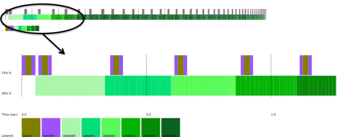
Figure 10. A trace of the Cholesky factorization on a multicore CPU with a single GPU K20c,
assigning the panel factorization task to the CPU (brown task) and the update to the GPU (green task) for a matrix of size 20,000.
as similarly equipped peers and assign them equivalent amounts of work. This na¨ıve strategy would cause the accelerator to be idle most of the time. In our model we propose to assign the latency-bound operations to the CPUs and the compute-intensive ones to accelerators. In order to support multi-way heterogeneous hardware, QUARK was extended with a mechanism for distributing tasks based on the individual capabilities of each device. For each device iand each kernel typek, extended version of QUARK maintains anαik parameter which corresponds
to the effective performance rate that can be achieved on that device. In the context of linear algebra algorithms, this means that we need an estimation of performance for Level 1, 2, and 3 BLAS operations. This can be done either by the developer during the implementation where the user gives a directive to QUARK which indicates that the kernel is either bandwidth-bound or compute-bound function (as shown in Algorithm 5 with a call toTask Flag Setwith aBLAS2
argument) or estimated according to the volume of data and the elapsed time of a kernel by the QUARK engine at runtime.
Figure 10 shows the execution trace of the Cholesky factorization on a single multicore CPU and a K20c GPU of System A (hardware labels and description is given in Section 7.1). We see that the memory-bound kernel (e.g., the panel factorization for the Cholesky algorithm) has been allocated to the CPU while the compute-bound kernel (e.g., the update performed by
of such a strategy is not only to hide the data transfer cost between the CPU and GPU (since it is overlapped with the GPU computation), but also to keep the GPU’s CUDA streams busy by providing enough tasks to execute. This is highlighted in Figure 10, where we can see that the panel of step 1 is quickly updated by the GPU and sent to the CPU to be factorized and sent back to the GPU, which is a perquisite to perform the trailing matrix update of step 1, before the GPU has already finished the update of trailing matrix of step 0, and so on.
However, it is clear that we can improve this further by fully utilizing all the available resources, particularly exploiting the idle time of the CPUs (white space in the trace). Based on the parameters defined above, we can compute a resource capability-weights for each task that reflects the cost of executing it on a specific device. This cost is based on the communication cost (if the data has to be moved) and on the type of computation (memory-bound or compute-bound) performed by the task. For a task that requires ann×ndata, we define its computation type to be from one of the Levels of BLAS (either 1, 2, or 3). Thus the two factors are simply defined as:
communication = n×n bandwidth computation =nk×αik
wherek is the Levelk BLAS
The capability-weights for a task is then the ratio of the total cost of the task on one resource versus the cost on another resource. For example, the capability-weights for the update operation (a Level 3 BLAS) from the execution shown in Figure 10 is around 1 : 10 which means that the GPU can execute 10 times as many update tasks as the CPU.
6.3. Greedy Scheduling Using Capability-Weights
As each task is inserted into the runtime, it is assigned to the resource with the largest remaining capability-weights. This greedy heuristic takes into account the capability-weights of the resource as well as the current number of waiting tasks preferred to be executed by this resource. For example, for the CPU, the panel tasks are memory-bound and thus are preferred to be executed always on the CPU side. The heuristic tries to maintain the ratios of the capability-weights across all the resources.
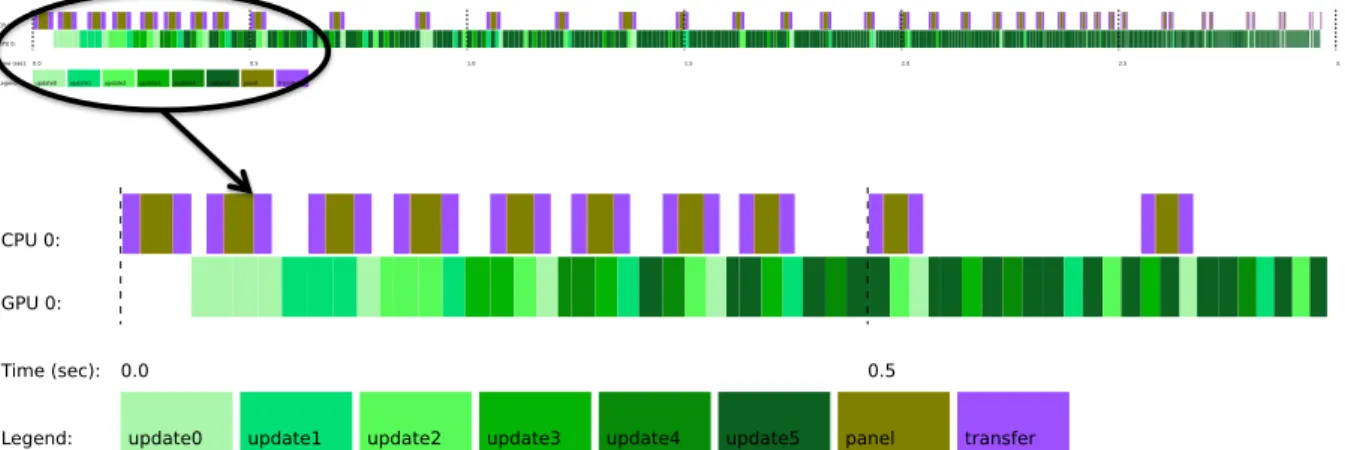
In Figure 11, we can see the effect of using capability-weights to assign a subset of the update tasks to the CPU. The GPU remains as busy as before, but now the CPU can contribute to the computation and does not have as much idle time as before. Careful management of the capability-weights ensures that the CPU does not take any work that would cause a delay to the GPU, since that would negatively affect the performance. We also plot in Figure 12 the performance gain obtained when using this technique. The graph shows that on a 16-core Sandy Bridge CPU, we can achieve a gain of around 100 Gflop/s (red curve) and 80 Gflop/s (blue curve) when enabling this technique when using a single Fermi M2090 and Kepler K20c GPU on System A and B, respectively (the hardware is described in§7.1).
6.4. Improved Task Priorities
Figure 11. A trace of the Cholesky factorization on 16-core, 2-socket Sandy Bridge CPU and a
K20c GPU, using capability-weights to distribute tasks.
2k 4k 6k 8k 10k 12k 14k 16k 18k 20k 22k 24k 26k
0
200
400
600
800
1000
1200
Matrix size
Gflop/s
DPOTRF using CW
DPOTRF no CW
DPOTRF using CW
DPOTRF no CW
Figure 12. Performance comparison of the Cholesky factorization when using the
capability-weights (CW) to distribute tasks among the heterogeneous hardware, on a node of 16 Sandy-Bridge CPU and either a Kepler (K20c) of system A “red curve” or a Fermi(M2090) of system B “blue curve”.
the panel factorization can be executed earlier. This increases the lookahead depth that the algorithm exposes, increasing parallelism so that there are more update tasks available to be executed by the device resources. Using priorities to improve lookahead results in approximately 5% improvement in the overall performance of the factorization. Figure 13 shows the update tasks being executed earlier in the trace.
Figure 13. Trace of the Cholesky factorization on multicore 16 Sandy Bridge CPU and a K20c
GPU, using priorities to improve lookahead.
6.5. Data Layout
When we proceed to the multiple accelerator setup, the data is initially distributed over all the accelerators in a 1-D block-column cyclic fashion, with an approximately equal number of columns assigned to each. Note that the data is allocated on each device as one contiguous memory block with the data being distributed as columns within the contiguous memory seg-ment. This contiguous data layout allows large update operations to take place over a number of columns via a single Level 3 BLAS operation, which is far more efficient than having multiple calls with block columns.
6.6. Hardware-Guided Data Distribution (HGDD)
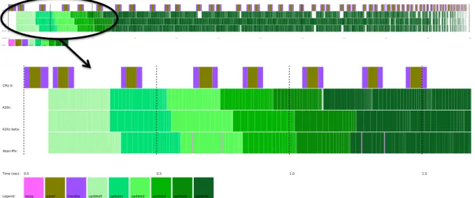
The experiments so far showed that the standard 1-D block cyclic data layout was hindering performance in heterogeneous multi-accelerator environments. Figure 14 shows the trace of the Cholesky factorization for a matrix of size 30,000 on System D (consisting of a Kepler K20c, a Xeon Phi (MIC) and Kepler K20-beta that has half the K20c performance). The trace shows that the execution flow is bound by the performance of the slowest machine (the beta K20, second row) and thus we expect lower performance on this machine.
Figure 14. Cholesky factorization trace on multicore CPU and multiple accelerators (a Kepler
K20c, a Xeon Phi, and an old K20-beta-release), using 1D block cyclic data distribution without enabling heterogeneous hardware-guided data distribution.
Figure 15. Cholesky factorization trace on multicore CPU and multiple accelerators (a Kepler
K20c, a Xeon Phi, and an old K20-beta-release), using the heterogeneous hardware-guided data distribution techniques (HGDD) to achieve higher hardware usage.
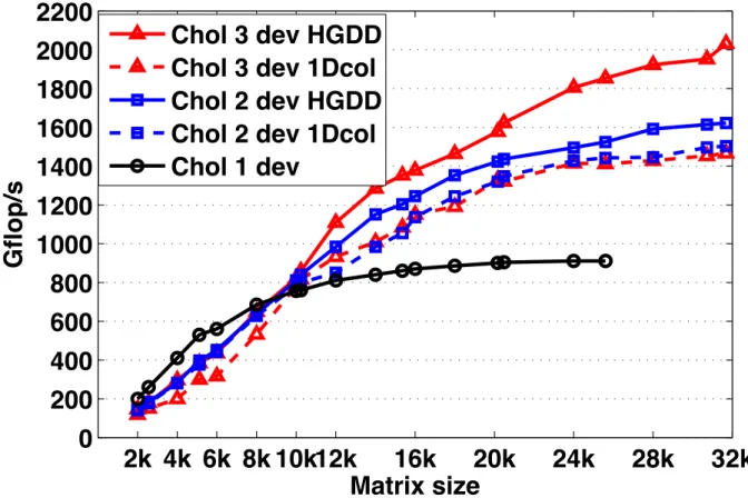
can notice that the standard distribution do not exhibit any speedup. The dashed red curve that represents the performance of the Cholesky factorization using the standard data distribution on the three devices of System D behaves closely and less efficient that the one obtained with the same standard distribution on two devices (dashed blue curve). This was expected, since adding one more device with lower capability may decrease the performance as it may slowdown the fast device. The blue and red curves in Figure 16 illustrate that the HGDD technique exhibits a very good scalability for both algorithms. The graph shows that the performance of the algorithm is not affected by the heterogeneity of the machine, our proposed implementation is appropriate to maintain a high usage of all the available hardware.
2k 4k 6k 8k 10k12k
16k
20k
24k
28k
32k
0
200
400
600
800
1000
1200
1400
1600
1800
2000
2200
Matrix size
Gflop/s
Chol 3 dev HGDD
Chol 3 dev 1Dcol
Chol 2 dev HGDD
Chol 2 dev 1Dcol
Chol 1 dev
Figure 16. Performance comparison of the Cholesky factorization when using the
hardware-guided data distribution techniques versus a 1-D block-column cyclic, on heterogeneous accel-erators consisting of a Kepler K20c (1dev), a Xeon Phi (2dev), and an old K20-beta-release (3dev).
6.7. Hardware-Specific Optimizations
One of the main enablers of good performance is optimizing the data communication between the host and accelerator. Another one is to redesign the kernels to exploit the inherent parallelism of the accelerator even by adding extra computational cost.
2k 4k 6k 8k 10k 12k 14k 16k 18k 20k 22k 24k 26k
0
200
400
600
800
1000
1200
1400
1600
1800
Matrix size
Gflop/s
QR 3dev (HGDD)
QR 3dev (1D
−
cyclic)
QR 2dev (HGDD)
QR 2dev (1D
−
cyclic)
QR 1dev
Figure 17. QR performance comparison for hardware-guided data distribution techniques vs.
1-D block-column cyclic, on heterogeneous accelerators consisting of a Kepler K20c (1dev), a Xeon Phi (2dev), and an old K20-beta-release (3dev).
6.7.1. Redesigning BLAS Kernels to Exploit Parallelism and Minimize the Memory Movement
The Hermitian rank-k update (SYRK) required by the Cholesky factorization implements the operation A(k)=A(k)−P P∗, whereA is annby nHermitian trailing matrix of stepk, and P is the result of the panel factorization done by the CPU. After distribution, the portion ofA on each accelerator no longer appears as a symmetric matrix, but instead has a ragged structure shown in Figure 18.
GPU 0 GPU 1
Figure 18.Block-cyclic data distribution. Shaded areas contain valid data. Dashed lines indicate
diagonal blocks.
up-date the remainder of each block column below the diagonal block. However, these small SYRK
operations have little parallelism and so are inefficient on an accelerator. This can be improved to some degree by using either multiple streams (GPU) or a pragma (MIC) to execute several
SYRKupdates simultaneously. However, because we have copied the data to the device, we can consider the space above the diagonal to be a scratch workspace. Thus, we update the entire block column, including the diagonal block, writing extra data into the upper triangle of the diagonal block, which is subsequently ignored. We do extra computation for the diagonal block, but gain efficiency overall by launching fewer BLAS kernels on the device and using the more efficient GEMM kernels, instead of smallSYRKkernels, resulting in overall 5-10% improvement in performance.
6.7.2. Improving Coalesced Data Access
The LU factorization uses the LASWP routine to swap two rows of the matrix. However, this simple data copy operation might drop the performance of such routines on accelerator architecture since it is recommended that a set of threads read coalescent data from the memory which is not the case for a row of the matrix. Such routine needs to be redesigned in order to overcome this issue. The device data on the GPU is transposed using a specialized GPU kernel, and is always stored in a transposed form, to allow coalesced read/write when the
LASWPfunction is involved. We note that the transpose does not affect any of the other kernels (GEMM,TRSM) required by the LU factorization. The coalesced reads and writes improve the performance of the LASWPfunction 1.6 times.
6.7.3. Enabling Specific Architecture Kernels
The size of the main Level 3 BLAS kernel that has to be executed on the devices is yet another critical parameter to tune. Every architecture has its own set of input problem sizes that achieve higher than average performance. In the context of one-sided algorithms, all the Level 3 BLAS operations depend on the size of the block panel. On the one hand, a small panel size lets the CPUs finish early but leads to lower Level 3 BLAS performance on the accelerator. On the other hand, a large panel size burdens the CPU and the CPU computation is too slow to be fully overlapped with the accelerator work. The panel size corresponds to a trade-off between the degree of parallelism and the amount of data reuse. In our model, we can easily tune this parameter or allow the runtime to autotune it by varying the panel size throughout the factorization.
6.7.4. Trading Extra Computation for Higher Performance Rate
Figure 19. Trace of Cholesky factorization on multicore CPU and multiple accelerators (up to
6 Kepler K20c).
7. Experimental Setup and Results
7.1. Hardware Description and SetupOur experiments were performed on a number of shared-memory systems available to us at the time of writing of this paper. They are representative of a vast class of servers and worksta-tions commonly used for computationally intensive workloads. We conducted our experiments on four different systems all of each equipped with an Intel multicore processor in a dual-socket configuration with 8-core Intel Xeon E5-2670 (Sandy Bridge) processors in a socket, each run-ning at 2.6 GHz. Each socket had 24 MiB of shared L3 cache, and each core had a private 256 KiB Level 2 and 64 KB Level 1 cache. The system is equipped with 52 GB of memory and the theoretical peak in double precision is 20.8 Gflop/s per core.
• System A is also equipped with six NVIDIA K20c cards with 5.1 GB per card running at 705 MHz, connected to the host via two PCIe I/O hubs at 6 GB/s bandwidth.
• System B is equipped with three NVIDIA M2090 cards with 5.3 GB per card running at 1.3 GHz, connected via two PCIe I/O hubs at 6 GB/s bandwidth.
• System C is also equipped with three Intel Xeon Phi cards with 15.8 GB per card running at 1.23 GHz, and achieving a double precision theoretical peak of 1180 Gflop/s, connected via four PCIe I/O hubs at 6 GB/s bandwidth.
• System D is a heterogeneous system equipped with a K20c, and a Intel Xeon Phi card as the ones described above, and also an old K20c beta release 3.8 GB running at 600 MHz. All are connected via four PCIe I/O hubs at 6 GB/s bandwidth.
A number of high performance software packages were used for the experiments. On the CPU side, we used the MKL (Math Kernel Library) [15]. On the Xeon Phi side, we used the MPSS 2.1.5889-16 as the software stack, icc 13.1.1 20130313 which comes with the Composer XE 2013.4.183 suite as the compiler, and finally on the GPU accelerator we used CUDA version 5.0.35.
7.2. Mixed MIC and GPU Results
2k4k 8k 12k16k20k24k28k32k36k40k 50k 60k 0
400 800 1200 1600 2000 2400 2800 3200 3600 4000 4400 4800 5200
Matrix size
Gflop/s
DPOTRF 6 K20c DPOTRF 4 K20c DPOTRF 3 K20c DPOTRF 2 K20c DPOTRF 1 K20c
Figure 20. Performance scalability of Cholesky factorization on multicore CPU and multiple
accelerators (up to 6 Kepler K20c).
2k4k6k8k 12k 16k 20k 24k 28k 32k 36k 40k 0
400 800 1200 1600 2000 2400
Matrix size
Gflop/s
DPOTRF_3 XeonPhi DPOTRF_2 XeonPhi DPOTRF_1 XeonPhi
Figure 21. Performance scalability of Cholesky factorization on multicore CPU and multiple
accelerators (up to 3 XeonPhi).
2k4k 8k 12k16k20k24k28k32k36k40k 48k 56k 0
400 800 1200 1600 2000 2400 2800 3200 3600 4000 4400 4800 5200
Matrix size
Gflop/s
DGETRF 6 K20c DGETRF 4 K20c DGETRF 3 K20c DGETRF 2 K20c DGETRF 1 K20c
Figure 22. Performance scalability of the LU decomposition on multicore CPU and multiple
accelerators (up to 6 Kepler K20c).
2k4k6k8k 12k 16k 20k 24k 28k 32k 36k 40k 0
400 800 1200 1600 2000 2400
Matrix size
Gflop/s
LU 3 XeonPhi LU 2 XeonPhi LU 1 XeonPhi
Figure 23. Performance scalability of the LU decomposition on multicore CPU and multiple
accelerators (up to 3 Xeon Phi).
2k4k 8k 12k16k20k24k28k32k36k40k 48k 56k 0
400 800 1200 1600 2000 2400 2800 3200 3600 4000 4400 4800
Matrix size
Gflop/s
DGEQRF 6 K20c DGEQRF 4 K20c DGEQRF 3 K20c DGEQRF 2 K20c DGEQRF 1 K20c
Figure 24. Performance scalability of the QR decomposition on multicore CPU and multiple
accelerators (up to 6 Kepler K20c).
2k4k6k8k 12k 16k 20k 24k 28k 32k 36k 40k 0
400 800 1200 1600 2000 2400
Matrix size
Gflop/s
QR 3 XeonPhi QR 2 XeonPhi QR 1 XeonPhi
Figure 25. Performance scalability of the QR decomposition on multicore CPU and multiple
accelerators (up to 3 Xeon Phi).