7
CONCURRENT ENGINEERING OF TOLERANCE SYNTHESIS AND
PROCESS SELECTION FOR PRODUCTS WITH MULTIPLE QUALITY
CHARACTERISTCS CONSIDERING PROCESS CAPABILITY
Mohamad Imron Mustajib
Manufacturing Systems Laboratory, Department of Industrial Engineering, University of Trunojoyo Madura, Kamal, Bangkalan 69162, Indonesia
E-mail: [email protected]
Abstract
The existences of variances that are very difficult to be removed from manufacturing processes provide significance of tolerance to the product quality characteristics target of customer functional requirement. Furthermore, quality loss incurred due to deviation of quality characteristics of the target with a specified tolerance. This article discusses the development of concurrent engineering optimization model of tolerance design and manufacturing process selection on product with multiple quality characteristics by minimizing total costs in the system, namely total manufacturing cost and quality loss cost as functions of tolerance, also rework and scrap costs. The considered multiple quality characteristics have interrelated tolerance chain. The formulation of proposed model is using mixed integer non linear programming as the method of solution finding. In order to validate of the model, this study presents a numerical example. It was found that optimal solution are achieved from proposed model in the numerical example.
Abstrak
Rekayasa Simultan Sintesis Toleransi dan Pemilihan Proses untuk Produk dengan Multi-karakteristik Kualitas
yang Mempertimbangkan Kapabilitas Proses. Keberadaan variansi yang sangat sulit untuk dihilangkan dalam
proses manufaktur memberikan peran penting adanya toleransi terhadap target karakteristik kualitas produk yang menjadi kebutuhan fungsional bagi konsumen. Selanjutnya timbul kerugian kualitas yang disebabkan oleh penyimpangan karakteristik kualitas dari target dengan toleransi yang ditetapkan. Makalah ini membahas pengembangan model optimisasi rekayasa simultan desain toleransi dan pemilihan proses manufaktur pada produk dengan multi karakteristik kualitas untuk meminimasi total ongkos dalam sistem, yaitu total ongkos manufaktur dan ongkos kerugian kualitas yang merupakan fungsi dari toleransi serta ongkos rework dan ongkos scrap. Karakteristik kualitas produk yang diperhatikan dalam penelitian ini memiliki rantai toleransi yang saling berkaitan (interrelated chain). Formulasi model yang dikembangkan menggunakan mixed integer non linear programming sebagai metode pencarian solusi.
Keywords: optimization model, quality loss, rework, scrap, tolerance
1.
Introduction
Tolerance synthesis is a critical issue in design and manufacturing stages, which affects both of product and process design because the tolerance is the bridge between product requirements and manufacturing cost [1]. Tolerance synthesis, which is also called tolerance allocation, is carried out in a direction opposite to tolerance analysis; from the tolerance of the function of interest to the individual tolerances [2]. According to Gryna et al. [3] tolerance is set by the engineering
design function to define minimum and maximum values allowable for the product to work properly. In quality engineering, tolerance allocation reflects a trade-off between customer requirements and the ability of producers to satisfy them. Thus, the loss of both customers and producers can be balanced.
considering the process capability of production. While tolerance synthesis at the process design/planning phase is more focused on the ease in performing the production process. Thus, in this stage the desired tolerances allocation is set as loose as possible. Meanwhile, during a production process, variance leads to imperfections of the product. Therefore, tolerance synthesis must be considered in both product and process design.
The aim of tolerance synthesis is to determine the maximum and minimum deviation limits of the product quality characteristics due to imperfections of the production process. Costs consideration and the capability of production process to tolerance allocation have made the problem become more complex. The tolerance values will affect the ability of components to be assembled into a final product (assembly), process selection, tooling, set-up costs, operator skills, inspection and measurement, scrap and rework. Loose tolerance facilitates implementation of the production process resulting in lower production costs. Consequently, if tolerance is too loose it will reduces the quality performance of the product. On the other hand, strict tolerance will improve product performance, but scrap and rework costs are higher. A lower process capability causes more deviation of quality characteristics from maximum and minimum limits. Thus, allocation of optimal tolerance values should take into account to quality loss and manufacturing cost by considering design and tolerance constraints and also other constraints [4]. Quality loss function has been introduced by Taguchi [5] in order to make it easy for designer to make trade-off between manufacturing and quality loss cost. Moreover, process (machine) selection problem in the planning process can be done by minimizing total cost of manufacturing and quality loss cost.
A major focus in tolerance design model was for a single quality characteristic by incorporating quality loss [4,6-9]. Recently, Mustajib and Irianto [10] propossed an integrated model for tolerance allocation and selection process in multi-stage processes. Meanwhile, the importance of determining tolerances for multiple quality characteristics products has been demonstrated by Lee and Tang [11], Chou and Chen [12], Huang et al. [13], and Peng et al. [14]. Furthermore, many researches [15-17] extended this work on assembly products with multiple quality characteristics based on statistical approach.
Statistical approach estimates the accumulation of tolerance (stack-up condition) on the assembled product, which is based on the fact that the probability of the component is at an extreme lapse very low tolerance [18]. The impact of this is not only on tighter tolerance assembled product with looser component
tolerances but also lower manufacturing cost. On the other hand, when the precision limit of the process and tolerance limits of final product are based on worst-case criteria it tends to require tighter component tolerances with relatively expensive manufacturing cost, compared with statistical approaches (root sum square criteria).
Altough statistical approaches improved performance, many researchers have not addresed the problem of process selection by considering process capability. Process capability indices, including Cp, Cpk, and Cpm, have been proposed in the manufacturing industry to provide numerical measures on whether a process is capable of reproducing items meeting the manufacturing quality requirement preset in the factory [19]. In addition, tolerance allocation could minimize rework and scrap costs, but most of the researches in tolerance synthesis did not consider the scrap and rework rates of the process resulted from allocated tolerance.
Based on those shortcomings of existing model of tolerance synthesis of multiple quality characteristics in previous studies and the need for reducing manufacturing cost, we propose the development of concurrent engineering optimization model of tolerance synthesis and process selection by considering process capability and non conformance rate; scrap and rework rates. The overall objective of the model is minimizing total cost of the system, i.e. manufacturing and quality costs. The development was carried out by enhancing on the model of previous study [8,9,11-14] with respect to process capability and statistical approaches, also taking into account the quality loss cost is a function of tolerance as well as rework and scrap cost.
2.
Methods
2 ) ( )
(y r y m
L = − (1)
with
2
t C
r = (2)
In Eq.1r is a constant that converts the characteristics become the characteristics of engineering costs which is the loss coefficient of the final product quality. This costant is estimated based on the cost of rework (C) where is required when quality characteristics of the final product y deviating from the target m, but still within an acceptable tolerance limits customers (t). Further determination of the optimal value of tolerance should pay attention to aspects of the quality loss cost L(t) and the manufacturing cost P(t) with respect to design constraints and tolerance of other constraints that are relevant. In Fig. 1, L(t) states the cost of quality loss as a function of tolerance, whereas P (t) states the cost of manufacturing as a function of tolerance. Furthermore, P(t) also states the overall cost of manufacturing on the quality characteristics with tolerance t.
Quality Characteristics. The problem, however, in Eq.
1 above is applied only for products with single quality characteristic, while for products with multiple quality characteristics the value of quality loss can be expanded [9]:
( ) (
Y Y M) (
TRY M)
L = − − (3)
Eq. 2 is general; it means that each of quality characteristics are not considered whether it is correlated or not. In Eq. 3 above, Y=[Y1,...Yq,...YQ]T
states the vector for the qth quality characteristic and the vector of the qth quality characteristic target is denoted by M=[M1,...Mq,...MQ]T, and R is r x r matrix for
constant of the qth quality characteristic.
The value of the qth quality characteristic (Yq) can be
estimated from the dimension of ith component. This relationship can be stated in Eq. [4]:
).
,
(
1 i Iq
q
f
K
K
K
Y
=
K
K
(4)Figure 1. The Solution Space for an Unconstrained Space [4]
The mean of nominal dimension of the ith component (Ki) is µ1,...µi,...µI. Expanding of right-hand side Eq. 4
in Taylor series around µ1,...µi,...µI, by ignoring the
higher order we obtained [21]:
∑
= ⎟⎟
⎟
⎠ ⎞
⎜ ⎜ ⎜
⎝ ⎛
Δ ∂ ∂ +
= I
i Ki
i i K
q Y q
M q Y
1 μ (5)
This study consider that each of components of the ith component (Ki) can be produced by alternative
processes 1,...j,...J, so that quality characteristic Yq=fq(K11,...Kij,...KIJ) in Eq. 5 become:
∑
= ∑= ⎟⎟⎟
⎟
⎠ ⎞
⎜⎜ ⎜ ⎜
⎝ ⎛
Δ ∂
∂ +
= I
i J
j Kij
i ij K
q Y q
M q Y
1 1 μ (6)
Furthermore, deviation of of the qth quality characteristic (Dq) can be estimated based on the difference between the qth quality characteristic (Yq)
with the qth quality characteristic target (Mq):
∑
= ⎟⎟
⎟
⎠ ⎞
⎜ ⎜ ⎜
⎝ ⎛
Δ ∂ ∂ = −
= I
i Ki
i i K
q Y q
M q Y q D
1 μ (7)
Thus, the vector of multiple quality characteristics deviation is D=[D1,...Dq,...DQ]T. Based on the vector of
multiple quality characteristics deviation, Eq. 3 can be written with Eq. 8 to evaluate the multivariate quality loss function with:
( )
D DTRDL = (8)
or
D R T D
C= (9)
Elements of R matrix can be calculated based on a basic correlation in Eq. 2 that are extended to be loss of multiple quality characteristics. This expansion is formulated with [9]:
r C p
q p
i
r i D r q D qi
R =
∑ =1 1∑=
) ( ) (
,
withr=1,2,K,p
(
p+1)
/2(10)
Rqi represents the qth row and the ith column in matrix
elements of R. When both set of product quality deviation of D (denoted by D q (r)) and vector of D i (r)
and quality loss cost (Cr) are known, then the matrix elements of R (denoted by Rqi) can be finded. In case
p=2, it is required three data sets for matrix elements. Let we consider again that Eq. 7 can be expressed as the variance of the qth quality characteristic (σq2) with:
∑
= ∑= ⎟⎟⎟ Δ
⎟
⎠ ⎞
⎜ ⎜ ⎜ ⎜
⎝ ⎛
∂ ∂ = I
i Kij
J j
ij ij K
q Y q
1
2 2
1 2
μ
ΔKi2 in Eq. 11 is nothing but the variance of the ith
component dimension that produced by the jth process (σij2) which is statistically can be written with:
2 1 2 1 2 ij I i J j ij ij K q Y q σ μ σ ∑ = ∑= ⎟⎟⎟ ⎟ ⎠ ⎞ ⎜ ⎜ ⎜ ⎜ ⎝ ⎛ ∂ ∂ = (12)
Eq. 12 is in accordance with the statistical criteria approach (root sum square criteria) which states that the dimension of assembly product consists of variance dimensional of its components. Furthermore, if we consider that the qth quality characteristic derived from one or more components of interrelated dimensions chain, then the covariance of the rth and rth quality characteristic can be finded by Eq. 13:
(
)
∑ = ∑= ⎟⎟⎟ ⎟ ⎠ ⎞ ⎜ ⎜ ⎜ ⎜ ⎝ ⎛ ∂ ∂ ∂ ∂ = I i ij J j ij ij K s Y ij ij K q Y s r Cov 1 2 2 1 2 , 2 σ μ μ σ σ (13)Variance for the ith component produced by the jth process (σij2) in Eq. 12 and 13 can be estimated by
considering process capability index (Cp):
i i LSL i USL i Cp σ 6 − = (14)
Where are USLi and LSLi state upper and lower specification limits of the ith component. By considering the tolerance of one side only, Eq. 14 can be simplified to obtain variances and relationships to the jth component tolerance (tj) in Eq 15:
( )
23 2 ⎟ ⎟ ⎠ ⎞ ⎜ ⎜ ⎝ ⎛ = ij Cp ij t ij t ij σ (15)
This research consider that on average process have a mean shift of 1.5σ. It is consistent with Motorola’s original Six Sigma program which stipulate that a process was said to be six sigma quality level when Cp=2 and Cpk=1.5. By assuming 1.5σ process shift, Taguchi process capability index can be obtained [20]:
Cp Cp
Cpm 0.5447
2 5 . 1 1 = ⎟ ⎠ ⎞ ⎜ ⎝ ⎛ − = σ σ (16)
Moreover, the variance of the qth quality characteristic in the Eq. 12 and 13 can be rewritten into Eq. 17 and 18 by substituting Eq. 15 into Eq. 12 and 13 as follows.
( )
I q Qi Cpmij
ij t I i ij ij K q Y ij t
q ∑ ∀ ∈
= ⎟ ⎟ ⎠ ⎞ ⎜ ⎜ ⎝ ⎛ ∑ = ⎟⎟⎟ ⎟ ⎠ ⎞ ⎜ ⎜ ⎜ ⎜ ⎝ ⎛ ∂ ∂ = 1 , 2 51 . 5 2 1 2 τ σ (17)
(
)
21 5.51
2 1 2 , 2 ∑ = ∑= ∂ ∂ ∂ ∂ = ⎟⎟ ⎠ ⎞ ⎜ ⎜ ⎝ ⎛ ⎟⎟ ⎟ ⎟ ⎠ ⎞ ⎜⎜ ⎜ ⎜ ⎝ ⎛ I
i Cpmij
ij t J j ij ij K s Y i ij K q Y s r Cov μ μ σ σ (18)
Meanwhile, the variance covariance matrix can be
expressed by
σ
q2 vector of parameter [11]:( )
(
)
(
)
(
)
(
)
⎥⎥ ⎥ ⎥ ⎥ ⎥ ⎦ ⎤ ⎢ ⎢ ⎢ ⎢ ⎢ ⎢ ⎣ ⎡ = 2 2 , 2 1 2 2 2 2 , 2 1 2 , 2 1 2 2 , 2 1 2 1 2 p p Cov Cov p Cov Cov t q V σ σ σ σ σ σ σ σ σ σ σ σ L L M O M M M L L (19)Quality loss cost. Expected cost of quality loss due to deviation of quality characteristic from its target can be estimated by tracking the variance covariance matrix [11]. Thus, the quality loss expectations in Eq. 3 can be calculated by tracing the variance covariance matrix based on Eq. 17 which can be formulated in Eq. 20.
( )
[ ]
Ltij Trace[
RV q( )
tij]
E = σ2 (20)
Cost of non conformance. The process alternatives and
tolerance allocation have possibility to produce non fonformance if the process variances are out from minimum and maximum values allowed. Costs of non conformance includes rework and scrap cost. By assuming that all variance for the ith component produced by the jth process are normally distributed, then the probability of non concormance (ḡij) is
determined by probability meets tolerance limits (gij): ij
g ij
g =1− (21)
If the product is not to meets tolerance (ḡij) is classified
into two types, namely: (1) ḡ1ij, for probability where
tolerance is not met owing to undersize, and (2) ḡ2ij, for
probability where tolerance is not met due to oversize.
Thus, for symmetric bilateral tolerance (see Fig 2), both of rework rate and scrap rate can be obtained by following equation:
ij
g
1 =g
2ij= .gij2 1
(22)
Model formulation. The objective function the model
is minimizing total costs (TC), which is the sum of manufacturing cost and quality costs. Quality costs includes quality loss cost and failure costs. The cost of failure arises when the dimensional tolerance cannot be met and results in component dimensions are undersized or oversized. In mechanical product, if the dimension is undersize at the features likes a hole, a step, a groove, and a slot, it is need to be reworked with rework cost, cr
ij. On the other hand, if the dimension is oversize, it is
need to be scrapped with certain of scrap cost, csij. If the
dimensional tolerance is bilateral, then probability process cannot meets the dimensional tolerance (ḡij)
due to oversized is equal to probability cannot meets the dimensional tolerance due to undersized component [22]. Therefore, complete model of the objective function can be expressed by Eq. 23. Meanwhile, all of the model constraints are formulated by Eq. 24 to 27 respectively.
( )
[
]
⎥
⎥
⎥
⎥
⎥
⎥
⎥
⎦
⎤
⎢
⎢
⎢
⎢
⎢
⎢
⎢
⎣
⎡
⎟⎟
⎠
⎞
⎜⎜
⎝
⎛
∑ = ∑= + ∑
= ∑=
+
+ ∑
= ∑= +
−
=
I J
j Xij
s ij g s ij C I J
j Xij
r ij g r ij C
ij X ij t q RV Trace
I J
j Cij Xij
ij t ij B e ij A
TC Min
1
i 1
1
i 1
2 1
i 1
σ (23)
subject to:
1) Quality spesification of design
Q q Yq Cpm
Yq t ij x ij Cpm
ij t I
i J
j Kij
q Y
∈ ∀ ≤
∑
= ∑= ⎟
⎟ ⎠ ⎞ ⎜ ⎜ ⎝ ⎛ ∂
∂
, 2 2
2
1 1
(24)
2) Process precision limits J j I i ij t ij t
tijmin≤ ≤ max,∀ ∈ ∀ ∈ (25)
3) Alternative process
I J
J∑=1Xij = ∀i∈ ,
1 (26)
4) Binary decision variables
[ ]
i I j Jij
X ∈0,1,∀ ∈ ,∀ ∈ (27)
Notations
i. Indexs:
q = qth quality characteristic i = ith component
j = jth process alternative Q = set of quality characteristics
I = set of components J = set of process alternatives ii. Decision variables:
Xij = 1, if the ith component is processed by
using jth process alternative. And 0, if not.
tij = tolerance of the ith component which is
produced by using jth process alternative
iii. Performance:
TC = total costs iv. Parameters:
Aij, Bij ,Cij = coefficients of cost-process tolerance
function for the ith component by using jth process alternative to generate tolerance tij
R = px ppositive definte matrix for quality loss constant the qth quality
characteristic
2
q
Vσ = vector parameter σq2 of the variance
covariance matrix
2
ij
σ = variance for the ith component produced by the jth process
Yq = qth quality characteristic
ij K
q Y ∂
∂ = partial derivative of qth quality characteristic with respect to ith component produced by the jth process ij
Cpm = Taguchi process capability index for the ith component produced by the jth process
Yq
Cpm = Taguchi process capability index for the qth quality characteristic
r ij
c
= rework cost for the ith component produced by the jth process sij
c
= scrap cost for for the ith component produced by the jth process tYq = tolerance design of qth qualitycharacteristic max
ij
t
= upper tolerance limit for the ith component produced by the jth process minij
t
= lower tolerance limit for the ith component produced by the jth process sij
g
= scrap rate of non conforming tospecification for the ith component produced by the jth process. r
ij
g
= rework rate of non conforming to3.
Results and Discussion
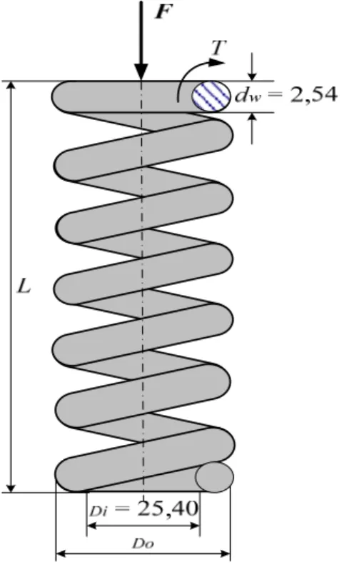
This section presents numerical example which is related to quality characteristic of one mechanical product, helical spring. This product is a type of compression spring made of round wire (diameter, dw),
wrapped in a straight line (length, L), cylindrical form with outer diameter Do and the number of coil springs is
n with constant distance between one coil with the others coils (Fig. 3). The use of helical spring is often found in a variety of equipments. In motor vehicles, the springs are usually used in suspension systems, engine valve springs and the clutch plate. Meanwhile, in the manufacturing process it is often used for the striper and the control valve of hydraulic and pneumatic systems. The springs are also widely used in small appliances such as on electrical switches, pen ballpoint, etc.
The main performance of a helical spring is an aspect that must be met within the design specifications. The purpose of helical spring design is to determine the dimensions of spring that can be operated at the limit load (F) and certain axial deflection (ΔL). Allowable stress depends on the material and dimensions of helical spring. Thus, the purpose of a helical spring design is quality specifications that are expected by the designers as customer needs.
Compressive force imposed axially on the helical spring (F) will cause axial deflection (ΔL). The relationship between the resulted force and deflection
Figure 3. Helical Spring
is called spring constant (k) or spring stiffness. Spring constant can be calculated by dividing the changing force and deflection.
L F k
Δ
= (28)
Because the loading is transmitted through wire spring, it will cause torsion. Therefore, the stress arising in the wire is the torsion shear stress (τ) which can be derived from the classical equation [23]:
p J Tc =
τ (29)
Meanwhile, the angular deflection (θ) on the wire can be calculated by using Eq. 30
G w d
n o FD
G w d
n o D o D F
p GJ
TL
4 2 16
4 32
2
= ⎟⎟ ⎠ ⎞ ⎜⎜ ⎝ ⎛
=
= π
π
θ (30)
Where T is the applied torque, G is the modulus of elasticity of spring material, and Jp states moment of polar inertia of wire material. Furthermore, axial deflection (ΔL) can be obtained by Eq. 31.
2
o D L=θ
Δ (31)
Note that the precision of spring outer diameter (Do) is
influenced by the precision of spring internal diameter (Di) and the spring wire diameter (dw). We consider that
the quality characteristic of outer diameter helical spring (Do) can be formulated by Eq. 32.
w d i D o
D = +2 (32)
By looking back to Eq. 28 as the basic equation represents spring performance, then the next quality characteristic helical spring which states the spring constant (k) or the spring stiffness can be formulated by Eq. 33 through substitution the value of θin Eq. 28 and 32 into Eq. 31
(
Di dw)
n w Gd k3 8
4
+
= (33)
Thus, both Eq. 32 and 33 above are the formulations for two quality characteristics of the helical spring. Furthermore, D0 is called the quality characteristic of Y1
and k is called the quality characteristic of Y2.
Partial derivative quality characteristic of Y1 and Y2 to
the component dimensions Di, dw, and n which is
resulted by process alternative (see Table 1) can be calculated as follows.
1 0
1
1 =
∂ ∂ = ∂
∂
i D D K
Y
Table 1. Cost Parameters, Tolerance Limits, and Non Conformance Rates
Cost Parameter Dimension Process
Alternative A B C
Lower Tolerance
Upper
Tolerance Scrap Rate
Rework Rate dw
1 1.581 78.735 1.44 0.018 0.80 0.003 0.001
2 14.132 7.262 1.44 0.020 0.82 0.002 0.002
Di
1 17.364 39.333 0.50 0.218 1.20 0.007 0.003
2 78.735 3.124 0.55 0.230 1.26 0.006 0.002
n 1 65.634 214.097 1.50 0.220 0.26 0.002 0.004
2 61.138 20.682 1.50 0.220 0.25 0.004 0.003
2 0 2 1 = ∂ ∂ = ∂ ∂ w d D K Y (35)
In similar manner, the partial derivatives for Y2 are as
follows:
(
)
4 0.256 437500
1
2 =−
+ − = ∂ ∂ = ∂ ∂ w d i D n w d i D k K Y (36)
(
)
(
)
3.5 4 4 37500 3 3 50000 2 2 = + − + = ∂ ∂ = ∂ ∂ w d i D n w d w d i D n w d w d k K Y (37)(
)
3 0.238 44 12500
3
2 =−
+ − = ∂ ∂ = ∂ ∂ w d i D n w d n k K Y (38)
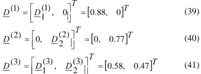
The data obtained from previous study [12], for example, are the number of coils (n ≈ 10), modulus of elasticity of helical spring material, G = 100.000 kg/mm, and quality tolerance of product design (Table 1). Suppose that the values of product design tolerances are D0=1.107 and k=1.106. Furthermore, the quality
characteristic of Y1 and Y2 deviate from their target
vector by values:
[
]
TT D
D (1), 0 0.88, 0
1 ) 1 ( = ⎥⎦ ⎤ ⎢⎣ ⎡ = (39)
[
]
TT D
D (2) 0, 0.77
2 , 0 ) 2 ( = ⎥⎦ ⎤ ⎢⎣ ⎡ = (40)
[
]
TT D D
D (3) 0.58, 0.47
2 , ) 3 ( 1 ) 3 ( = ⎥⎦ ⎤ ⎢⎣ ⎡ = (41)
will result in product failure and cause a loss of 60$.
Furthermore, elements of the quality loss constant matrix can be obtained through Eq. 10.
48 . 77 2 88 . 0 60 2 ) 1 ( 1 1
11 = =
⎟ ⎠ ⎞ ⎜ ⎝ ⎛ = D C R (42) 20 . 101 2 77 . 0 60 2 ) 2 ( 2 2
22 = =
⎟ ⎠ ⎞ ⎜ ⎝ ⎛ = D C R (43)
Table 2. The Optimal Solutions of Three Process
Capability Scenarios
Cpm
0.888 1 1.109
t1 0.031 0.032 0.032
t2 0.218 0.230 0.218
t3 0.220 0.220 0.220
X1 1 2 1
X2 1 2 1
X3 1 1 1
TC 19.40203 18.4911 16.38516
( ) ( ) ( )
( ) 21.24
47 . 0 58 . 0 2 2 77 , 0 2 47 , 0 60 2 88 , 0 2 58 , 0 60 60 ) 3 ( 2 3 1 2 2 2 2 2 3 2 1 2 1 1 2 3 1 1 3 21 12 = × × ⎥⎦ ⎤ ⎢⎣ ⎡ − − = ⎟ ⎠ ⎞ ⎜ ⎝ ⎛ ⎥ ⎥ ⎦ ⎤ ⎢ ⎢ ⎣ ⎡ ⎟ ⎠ ⎞ ⎜ ⎝ ⎛ ⎟ ⎠ ⎞ ⎜ ⎝ ⎛ − ⎟ ⎠ ⎞ ⎜ ⎝ ⎛ ⎟ ⎠ ⎞ ⎜ ⎝ ⎛ − = = D D D D C D D C C R R (44)
Meanwhile, elements of the variance covariance matrix can be obtained through Eq. 17 and 18. In case Cpm=1, the expected of quality lost cost can be generated by using of MathCAD 14.0 software as follows:
( )
[ ]
2 32 72 . 123 2 31 72 . 123 2 22 23 . 147 2 21 66 . 144 2 12 93 . 73 2 11 36 . 71 t t t t t t ij t L E + + + + + = (45)Finally, decision variables of the optimization model of tolerance design and manufacturing process selection on helical spring can be obtained by solved in the proposed model by using the LINGO software package. The optimal tolerances and process with another two process capability scenarios are given in Table 2.
4.
Conclusion
This study proposed the development of concurrent engineering optimization model of tolerance synthesis and process selection by considering process capability and costs of non conformance. The objective of the model is minimizing total cost of the system, i.e. manufacturing and quality costs. Formulation of the model developed using mixed integer non linear programming as the method of solution finding. In order to validate of the developed model, this study presents a numerical example. It was found that optimal solution are resulted from proposed model in the numerical example. The optimization results data in indicate that there were relationship between process capability and total costs in the system. Meanwhile, the impact of process capability increasing have significantly reduced total cost. Moreover, the changes of process capability have changed tolerance allocation and selected process. In summarize, this finding is promising and should be explored with other methods for finding better optimal solutions. It is possible to use computational intelligence to enhance the method of solution finding for proposed model.
References
[1] H.C. Zhang, Advanced Tolerancing Techniques, Willey Series in Engineering Design and Automation, John Willey & Sons, New York, USA, 1997, p. 207
[2] Y.S. Hong, T.C. Chang, Int. J. Prod. Res. 40/11 (2002) 2425.
[3] M.F. Gryna, R.C.H. Chua, J.A. DeFeo, Juran’s Quality Planning and Analysis: For Enterprises Quality, 5th ed., McGraw-Hill, Inc., New York 2007, p.655.
[4] C.X. Feng, J. Wang, J.S. Wang, Comput. Ind. Eng. 40 (2001) 15.
[5] G. Taguchi, S. Chowdhury, Y. Wu, Taguchi’s Quality Engineering Handbook, John Willey & Sons. Inc., Hoboken, New Jersey, USA, 2005, p.134.
[6] S. Shin, B.R. Cho, Eng. Optimiz. 40/11 (2008) 989. [7] P. Muthu, V. Dhanalakshmi, K. Sankaranara-yanasamy, Int. J. Adv. Manuf. Tech. 44 (2010) 1154.
[8] K. Sivakumar, C. Balamurugan, S. Ramabalan, Int. J. Adv. Manuf. Technol. 53 (2011) 711. doi: 10.1007/s00170-010-2871-4.
[9] K. Sivakumar, C. Balamurugan, S. Ramabalan, Comput. Aided Design, 43 (2011) p.207.
[10]M.I. Mustajib, D. Irianto, J. Adv. Manuf. Sys. 9/1 (2010) 31. doi: 10.1142/S02196867000-1788. [11]C.L. Lee, G.R. Tang, Mech. Mach. Theory. 35
(2000) 1658.
[12]C.Y. Chou, C.H. Chen, Int. J. Prod. Econ. 70 (2001) 279.
[13]M.F. Huang, Y.R. Zhong, Z.G. Xu, Int. J. Adv. Manuf. Technol. 25 (2005) 714.
[14]H.P. Peng, X.Q. Jiang, X.J. Liu, Int. J. Adv. Manuf. Technol. 39/1 (2007) 1. doi:10.1007/s00170-007-1205-7.
[15]P.K. Singh, S.C. Jain, P.K. Jain, Comput. Ind. 56 (2005) 179.
[16]H.P. Peng, X.Q. Jiang, X. J. Liu, Int. J. Prod. Res. 46/24 (2008) 6963.
[17]I. González, I. Sánchez, Mech. Mach. Theory. 44 (2009) 1097.
[18]S.S. Lin, H.P. Wang, C. Zhang, In: H.C. Zhang, Advanced Tolerancing Techniques, Willey Series in Engineering Design and Automation, John Willey & Sons, Inc., New York, USA, 1997, p.261. [19]W.L. Pearn, M.H. Shu, Int. J. Adv. Manuf.
Technol. 23 (2005) 116.
[20]C.X. Feng, R. Balusu, Con. Innov. Design Manuf. 103 (1999) 1.
[21]D.C. Montgomery, Introduction to Statistical Quality Control, 4th ed., John Willey & Sons, Inc., Hoboken, New Jersey, USA, 2001, p.392.
[22]Y.H. Lee, C.C. Wei, C.B. Chen, C.H. Tsai, Eng. Optimiz. 32 (2000) 619.