VI International Conference on Computational Methods in Marine Engineering MARINE 2015 F. Salvatore, R. Broglia and R. Muscari (Eds)
COMPARISON OF THE EXTREME RESPONSES FROM DIFFERENT
METHODS OF SIMULATING WAVE KINEMATICS
N.I. MOHD ZAKI*, M.K. ABU HUSAINa AND G. NAJAFIANb
* UTM Razak School of Engineering and Advanced Technology Universiti Teknologi Malaysia
Jalan Semarak, 54100 Kuala Lumpur, Malaysia e-mail: [email protected]
a UTM Razak School of Engineering and Advanced Technology Universiti Teknologi Malaysia
Jalan Semarak, 54100 Kuala Lumpur, Malaysia e-mail: [email protected]
b School of Engineering
The Quadrangle, The University of Liverpool Liverpool, L69 3GH, United Kingdom
e-mail: [email protected]
Key words: Linear Random Wave Theory, Kinematics, Surface Zone, Stretching Method
Abstract. Linear random wave theory (LRWT) is frequently used to simulate water particle kinematics at different nodes of an offshore structure from a reference surface elevation record. However, it is well known that LRWT leads to water particle kinematics with exaggerated high-frequency components in the vicinity of mean water level (MWL). Methods have been introduced to overcome this problem of high kinematics above the MWL consists of using linear wave theory (such as Wheeler, vertical stretching, effective node elevation and effective water depth methods) can be used to provide a more realistic representation of near-surface wave kinematics. There is promising as there is some evidence that the water particle kinematics from the Wheeler method are underestimated and that those from the vertical stretching method are somewhat exaggerated. In this paper, the comparisons of the probability distributions of extreme values from different methods of simulation wave kinematics are investigated by using Monte Carlo simulation procedure.
1 INTRODUCTION
For an offshore structure, wind, wave and gravitational forces are all important sources of loading. The dominant load, however, is normally due to wind-generated random waves. It is therefore of great importance to calculate the wave loads on the structure accurately.
Morison’s equation [1] is frequently used to calculate wave loads on the cylindrical members of an offshore structure from the wave-induced water particle kinematics. It can therefore be concluded that the accurate estimation of wave-induced water particle kinematics is a key step for accurate prediction of wave loads on the structure.
Linear random wave theory (LRWT) is frequently used to calculate wave-induced water particle kinematics at different nodes of an offshore structure from a simulated surface elevation record by using appropriate transfer functions. It is, however, well known that linear wave theory gives unacceptable results near the free surface, especially for high- frequency wave components. To overcome this deficiency, a common industry practice for evaluation of wave kinematics in the free surface zone consists of using linear wave theory in conjunction with empirical techniques to provide a more realistic representation of near-surface wave kinematics. The empirical techniques popular in the offshore industry include Wheeler stretching [2], linear extrapolation and delta stretching [3] and vertical stretching [4]. Couch and Conte [5] offer a review of these techniques.
More accurate results can be obtained from the Hybrid Wave Model, which is a second order random wave theory [6]. In one study [7], water particle kinematics near the free surface zone from some laboratory experiments were compared with predictions from different methods. It was concluded that the Hybrid Wave Model was more accurate than either the Wheeler method or the linear extrapolation technique. The results indicated that while the linear extrapolation method overestimated the water particle kinematics, the reverse was true for the Wheeler method. Longridge et al [8] made similar conclusions from analysis of laboratory data. They also concluded that both the Wheeler and the linear extrapolation methods are sensitive to the cut-off frequency of the surface elevation frequency spectrum. In other words, they lead to exaggerated water particle kinematics for high-frequency wave components. Donelan et al [9] also concluded from analysis of laboratory data that both direct application of LRWT and the linear extrapolation method greatly overestimate water particle velocities in the near surface zone and that they are both sensitive to the choice of cut-off frequency.
Couch and Conte [5] used water particle kinematics from the Hybrid Wave Model together with those from various stretching techniques to compare the predicted response of the Cognac platform with corresponding measured response data. They concluded that the Hybrid Wave Model leads to more accurate response predictions and that the Wheeler method was better than delta and vertical stretching techniques, which overestimate the response particularly at high frequencies. This conclusion is different from other studies, which indicate that the Wheeler method underestimates the water particle kinematics under wave
crests. It should, however, be noted that Morison’s drag and inertia coefficients used in this study were 0.90 and 2.3, respectively, which are somewhat high, and that the response evaluation did not account for variation of wave kinematics in the horizontal direction. The effect of wave directionality was not considered, either. It is, therefore, reasonable to conclude that the response has been overestimated due to the foregoing reasons and that this has compensated for the underestimation of water particle kinematics by the Wheeler method. Although more data is required to make reliable conclusions, it is generally believed that the Wheeler stretching technique underestimates the water particle kinematics under wave crests while other stretching methods tend to overestimate it. It is therefore desirable to come up with a method that resolves this problem. While the Hybrid wave model is more accurate, it is computationally very demanding and is mostly suitable for research purposes. Ideally, a
modified form of LRWT which could possibly lead to more accurate results compared with other stretching methods is required. To this end, two new methods, the effective node elevation and the effective water depth methods, have been introduced in this study [10,11]. The results indicate that the water particle kinematics predicted from these methods lie between corresponding values from the Wheeler and the vertical stretching methods. Ideally, comparisons with high-quality laboratory and field data, or corresponding results from the more accurate Hybrid wave model, are necessary to determine the level of accuracy of the proposed procedures in comparison with other techniques.
In this paper, the extreme structural responses for three different sea states and zero-current cases are calculated from four different methods of simulating water particle kinematics (vertical stretching, Wheeler stretching, effective node elevation and effective water depth methods) to investigate by how much they differ from each other. It is shown that the Wheeler and the vertical stretching methods, both popular in the industry, lead to significantly different estimates of the 100-year responses. Furthermore, two new methods for predicting water particle kinematics are introduced whose predicted 100-year responses lie between those from the Wheeler and the vertical stretching methods, and hence may be considered to be more appropriate for practical application.
2 TEST STRUCTURE AND RESPONSES
The test structure used in this paper is a fixed platform in a water depth of 110m. The general outline of the platform is shown in Figure 1. The platform is composed of four vertical legs, where the diameter of each leg is 1.5m with a wall thickness of 40mm. As shown in the figure, the distributed hydrodynamic load on each leg is represented by 30 point loads so that the total number of nodal loads on the four legs is 120. The dimensions of the platform deck are 35m*38m. The member surfaces were assumed to be rough and hence the drag and inertia coefficients were taken to be 1.05 and 1.20, respectively. The total mass of the topsides and the four legs (including the added hydrodynamic mass for the four legs of the structure) is 17665 Tonnes.
The foregoing test structures were subjected to various uni-directional sea-states simulated from Pierson–Moskowitz (P–M) frequency spectrum. The waves were assumed to propagate in the global Y direction (Figure 1). In this study, the following definition of the P–M spectrum [12] has been used:
𝐺𝐺𝜂𝜂𝜂𝜂(𝑓𝑓) = 𝐻𝐻𝑠𝑠 2
4𝜋𝜋𝑇𝑇𝑧𝑧4𝑓𝑓5 𝑒𝑒𝑒𝑒𝑒𝑒 (−
1
𝜋𝜋𝑇𝑇𝑧𝑧4𝑓𝑓4) (1)
where Gηη is the surface elevation frequency spectrum, Hs is the significant waveheight in
meters, Tz is the mean zero-upcrossing period in second and f is the wave frequency in Hz,. Surface elevation and corresponding water particle kinematics at different structural nodes were simulated according to linear random wave theory (LRWT). All the water particle kinematics have been multiplied by a wave kinematics factor of 0.95 to account for wave directionality in the sea. The mean zero-upcrossing period (in seconds) for each sea state was
taken to be 𝑇𝑇𝑧𝑧 = 3.55√𝐻𝐻𝑠𝑠with Hs denoting the significant waveheight in meters.
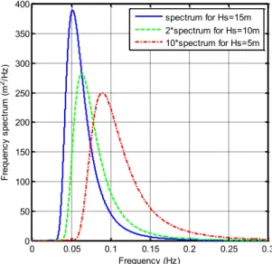
Furthermore, each response has been calculated for three different environmental conditions represented by Hs = 15m, 10m, and 5m, respectively. Surface elevation frequency spectra for
Hs = 15m, 10m and 5m are shown in Figure 2. The following responses were chosen for investigation: base shear and overturning moment.
Figure 1: Schematic diagram of the test structures.
Figure 2: Water surface elevation frequency spectra for three different sea states.
0 0.05 0.1 0.15 0.2 0.25 0.3
0 50 100 150 200 250 300 350 400
Frequency (Hz)
Fr
equenc
y s
pec
trum
(m
2/Hz
)
spectrum for Hs=15m 2*spectrum for Hs=10m 10*spectrum for Hs=5m
3 WAVE LOADING ON CYLINDRICAL MEMBERS OF OFFSHORE STRUCTURES
According to Morison’s equation, the wave-induced horizontal force per unit length on a vertical submerged cylinder (cylinder diameter / wavelength < 1/5) is the sum of a nonlinear drag component and a linear inertial component. That is,
𝐹𝐹(𝑡𝑡) =𝐹𝐹𝑑𝑑𝑑𝑑𝑑𝑑𝑑𝑑(𝑡𝑡) +𝐹𝐹𝑖𝑖𝑖𝑖𝑖𝑖𝑑𝑑𝑖𝑖𝑖𝑖𝑑𝑑 (𝑡𝑡) (2)
where drag and inertial components of fluid loading are, respectively, defined as
𝐹𝐹𝑑𝑑𝑑𝑑𝑑𝑑𝑑𝑑(𝑡𝑡) =𝑘𝑘𝑑𝑑𝑢𝑢(𝑡𝑡)|𝑢𝑢(𝑡𝑡)| (3)
𝐹𝐹𝑖𝑖𝑖𝑖𝑖𝑖𝑑𝑑𝑖𝑖𝑖𝑖𝑑𝑑(𝑡𝑡) =𝑘𝑘𝑖𝑖𝑢𝑢̇(𝑡𝑡) (4)
𝑘𝑘𝑑𝑑=12𝐶𝐶𝑑𝑑𝜌𝜌𝜌𝜌 and 𝑘𝑘𝑖𝑖=14𝐶𝐶𝑚𝑚𝜌𝜌𝜌𝜌𝜌𝜌2 (5)
where Cd and Cm are empirical drag and inertia coefficients; ρ is the fluid density; D is the leg cylinder diameter; and u(𝑡𝑡) and 𝑢𝑢̇(𝑡𝑡) are the horizontal component of water particle velocity
and acceleration, respectively. Further details about Morison’s equation can be found in
Sarpkaya and Isaacson [13] and Moe [14]. The assumption made in this paper is that
Morison’s equation with constant Cd and Cm values can adequately describe the in-line wave forces for a given sea state.
4 EVALUATION OF QUASI-STATIC RESPONSE BY TIME SIMULATION PROCEDURE
In summary, the steps taken to calculate the quasi-static response are as follows:
1. Assume a suitable surface elevation frequency spectrum, such as the Pierson-Moskowitz spectrum defined by its significant wave height, Hs and mean zero-upcrossing period, Tz. 2. Use linear random wave theory (LRWT) to simulate a surface elevation record at an
arbitrary reference point from the given frequency spectrum for a given period of time (4.5 hours in this study). According to LRWT, uni-directional seas can be modelled as the sum of a large number of progressive linear waves (wavelets) of different amplitudes travelling in the same direction with random phase angles [15]. Then, the surface elevation at point y
at time t can be modelled as:
𝜂𝜂(𝑦𝑦,𝑡𝑡) =∑ 𝐴𝐴𝑖𝑖cos(2𝜌𝜌𝑓𝑓𝑖𝑖𝑡𝑡 − 𝑘𝑘𝑖𝑖𝑦𝑦 − 𝜑𝜑𝑖𝑖) 𝑁𝑁𝑁𝑁
𝑖𝑖=1
(6)
where 𝑁𝑁𝑁𝑁 is the total number of wavelets used in the simulation, 𝑓𝑓𝑖𝑖 are a set of
equally-spaced discrete wave frequencies and 𝑘𝑘𝑖𝑖 are their associated wavenumbers. Parameter 𝜑𝜑𝑖𝑖 is
a random phase angle distributed uniformly in the range 0 <𝜑𝜑𝑖𝑖 < 2𝜌𝜌, and 𝐴𝐴𝑖𝑖 is
determined by one of the following two methods: (1) Deterministic Spectral Amplitude technique (DSA) and (2) Non-Deterministic Spectral Amplitude (NSA) technique. That is,
(𝐴𝐴𝑖𝑖)𝑁𝑁𝑁𝑁𝑁𝑁= (𝐴𝐴𝑖𝑖)𝐷𝐷𝑁𝑁𝑁𝑁∗ √𝑔𝑔𝑖𝑖 2+ℎ
𝑖𝑖 2
2 (8)
where 𝐺𝐺𝜂𝜂𝜂𝜂(𝑓𝑓) is the one-sided surface elevation frequency spectrum and Δ𝑓𝑓 is the frequency interval. Parameters 𝑔𝑔𝑖𝑖 and ℎ𝑖𝑖 are two independent and standardised Gaussian random variables. Rice [16] has shown that when NW approaches infinity, the two models will be equivalent to each other. The differences between the two techniques for finite values of NW have been discussed in Tucker et al [17), Grigoriu [18] and Morooka and Yokoo [19]. The NSA technique is more robust and hence has been used in this study. 3. Calculate wave-induced water particle kinematics at different nodes from the surface
elevation record by using appropriate transfer functions from linear wave theory. All empirical wave stretching techniques discussed in previous section were adopted for comparison purposes.
4. Calculate the drag and inertial components of Morison loads at each node accounting for load intermittency in the splash zone.
5. Calculate the drag-induced, 𝑅𝑅̃𝑑𝑑 and inertia-induced, 𝑅𝑅̃𝑖𝑖 components of the response (quasi-static base shear and overturning moment in this study). As the structural system is assumed to be linear, the total response would then be equal to the sum of the foregoing two components.
5 DERIVATION OF PROBABILITY DISTRIBUTION OF RESPONSE EXTREME VALUES BY THE MONTE CARLO PROCEDURE
For short-term distribution, use the procedure in Section 4 to simulate a response record from a simulated surface elevation record and determine its extreme value. Then repeat the process many times to generate a large sample of response extreme values. Rank all the simulated extreme values from smallest to largest. Then use the following plotting position equation for the Gumbel distribution [17] to estimate the value of the probability distribution for each of the ranked extreme values.
𝑃𝑃𝑃𝑃𝑃𝑃𝑃𝑃(𝑃𝑃𝑚𝑚𝑚𝑚𝑚𝑚<𝑞𝑞𝑛𝑛) = 𝑃𝑃𝑟𝑟𝑚𝑚𝑚𝑚𝑚𝑚(𝑞𝑞𝑛𝑛)≈
𝑛𝑛 −0.44
𝑁𝑁+ 0.12 , 𝑛𝑛= 1, 2, 3, … ,𝑁𝑁 (9)
where rmax denotes the response extreme value, qn is the nth smallest simulated extreme value, and finally N is the total number of simulated extreme values.
6 REVIEW OF EXISTING METHODS OF WAVE KINEMATICS
According to LRWT, uni-directional seas can be modelled as the sum of a large number of progressive linear waves (wavelets) of different amplitudes travelling in the same direction with random phase angles [15]. Then, the surface elevation (𝜂𝜂) at point x and time t can be modelled as:
𝜂𝜂(𝑥𝑥,𝑡𝑡) =∑ 𝜂𝜂𝑖𝑖(𝑥𝑥,𝑡𝑡) 𝑁𝑁𝑁𝑁 𝑖𝑖=1
∑ 𝐴𝐴𝑖𝑖 𝑐𝑐𝑃𝑃𝑐𝑐(2𝜋𝜋𝑓𝑓𝑖𝑖𝑡𝑡 − 𝑘𝑘𝑖𝑖𝑥𝑥 − 𝜑𝜑𝑖𝑖) 𝑁𝑁𝑁𝑁
𝑖𝑖=1
where NW is the total number of wavelets used in the simulation, fi are a set of discrete wave frequencies (Hz) and ki are their associated wave numbers. Parameter i is a random phase
angle distributed uniformly in the range 0 < i < 2, and Ai is the amplitude of the ith wave component. The horizontal water particle velocity (u) at a point with elevation (z) from mean water level (MWL) (assumed to be positive upwards) would then be equal to
𝑢𝑢(𝑥𝑥,𝑧𝑧,𝑡𝑡) =∑ 𝑢𝑢𝑖𝑖(𝑥𝑥,𝑧𝑧,𝑡𝑡) 𝑁𝑁𝑁𝑁
𝑖𝑖=1
(11) 𝑢𝑢𝑖𝑖(𝑥𝑥,𝑧𝑧,𝑡𝑡) =𝐴𝐴𝑖𝑖(2𝜋𝜋𝑓𝑓𝑖𝑖)cosh[sinh(𝑘𝑘𝑖𝑖(𝑘𝑘𝑑𝑑+𝑧𝑧)]
𝑖𝑖𝑑𝑑) cos(2𝜋𝜋𝑓𝑓𝑖𝑖𝑡𝑡 − 𝑘𝑘𝑖𝑖𝑥𝑥 − 𝜑𝜑𝑖𝑖) (12)
where d is the (mean) water depth. For high-frequency components, the wave length would be small and deep water condition would apply; therefore, the above equation can be simplified to
𝑢𝑢𝑖𝑖(𝑥𝑥,𝑧𝑧,𝑡𝑡) =𝐴𝐴𝑖𝑖(2𝜋𝜋𝑓𝑓𝑖𝑖)𝑒𝑒𝑘𝑘𝑖𝑖𝑧𝑧cos (2𝜋𝜋𝑓𝑓𝑖𝑖𝑡𝑡 − 𝑘𝑘𝑖𝑖𝑥𝑥 − 𝜑𝜑𝑖𝑖) (13)
The value of ekizis always smaller than unity for negative z values (points below the MWL); however, it grows very rapidly for high k and z values. This would lead to substantial high- frequency components of water particle kinematics at points above the MWL [20].
6.1 Vertical stretching method
As previously mentioned, various techniques have been developed to avoid this problem. The simplest one is the vertical stretching method [4]. In this method, water particle kinematics at points below MWL are calculated from (standard) LRWT, but water particle kinematics above the MWL are taken to be equal to their corresponding values at MWL. In other words, the following relationship is assumed to be valid.
𝑢𝑢(𝑥𝑥,𝑧𝑧,𝑡𝑡) =𝑢𝑢(𝑥𝑥, 0,𝑡𝑡), 𝑧𝑧> 0 (14)
6.2 Wheeler stretching method
In the Wheeler stretching method [2], the following equation is used to replace the vertical coordinate z with an equivalent node elevation which is always negative. That is,
𝑧𝑧′(𝑥𝑥,𝑡𝑡) =𝑑𝑑 𝑑𝑑+𝑧𝑧
𝑑𝑑+𝜂𝜂(𝑥𝑥,𝑡𝑡)− 𝑑𝑑 (15)
where η is the instantaneous surface elevation at point x and time t. It should be clear from the above equation that 𝑧𝑧′changes with time and that it is always negative when the point under consideration is inundated, that is when 𝜂𝜂 > 𝑧𝑧. When the surface elevation is below the point,
𝑧𝑧′ would be positive, but then, the water particle kinematics must be set equal to zero as the surface elevation is below the point. Therefore, the problem with rapid growth of water particle kinematics for high- frequency wavelets would not arise in the case of Wheeler approach. However, since 𝑧𝑧′ is a function of time, a transfer function could not be established to convert the surface elevation to water particle kinematics. Therefore, water particle kinematics for each wavelet must be calculated separately, and then, the contributions from all
wavelets must be added up to calculate the water particle kinematics due to all wavelets. This is in contrast with the LRWT, where transfer function (and hence the very efficient Fast Fourier Transform (FFT) technique) can be used to calculate water particle kinematics from the reference surface elevation record.
6.3 Effective node elevation method
It is, therefore, desirable to introduce an effective node elevation, 𝑧𝑧𝑒𝑒 [10] which is
negative but unlike that of the Wheeler method is of constant value. This was the basis of the effective node elevation method. In this technique, the constant effective node elevation, 𝑧𝑧𝑒𝑒 is
taken to be the average value of 𝑧𝑧′ when the node is inundated; in other words, when 𝜂𝜂 ≥ 𝑧𝑧. According to LRWT, η is a mean-zero Gaussian random variable whose standard deviation
(𝜎𝜎𝜂𝜂) is equal to Hs/4, where Hs is the significant wave height of the sea state. Therefore, the
probability density function of the surface elevation is equal to
𝑝𝑝(𝜂𝜂) = 1
√2𝜋𝜋𝜎𝜎𝜂𝜂𝑒𝑒
−𝜂𝜂2
2𝜎𝜎𝜂𝜂2 (16)
Then, the average value of 𝑧𝑧′ (referred to as the effective node elevation), when 𝜂𝜂 ≥ 𝑧𝑧, would be equal to
𝑧𝑧𝑒𝑒=𝐸𝐸[𝑧𝑧′|𝜂𝜂 ≥ 𝑧𝑧] =∫ 𝑧𝑧
′(𝜂𝜂)𝑝𝑝(𝜂𝜂)𝑑𝑑𝜂𝜂 ∞
𝑧𝑧
∫ 𝑝𝑝𝑧𝑧∞ (𝜂𝜂)𝑑𝑑𝜂𝜂 (17)
where
𝑧𝑧′(𝜂𝜂) =𝑑𝑑𝑑𝑑+𝑧𝑧
𝑑𝑑+𝜂𝜂 − 𝑑𝑑 (18)
6.4 Effective water depth method
In the effective water depth method, de [11] is taken as the average value of the surface elevation above sea bed when the node is inundated; in other words, when 𝜂𝜂 ≥ 𝑧𝑧. The effective water depth for a particular node is then equal to,
𝑑𝑑𝑒𝑒=𝑑𝑑+𝐸𝐸[𝜂𝜂|𝜂𝜂 ≥ 𝑧𝑧] =𝑑𝑑+∫ 𝜂𝜂𝑝𝑝
(𝜂𝜂)𝑑𝑑𝜂𝜂
∞ 𝑧𝑧
∫ 𝑝𝑝𝑧𝑧∞ (𝜂𝜂)𝑑𝑑𝜂𝜂 (19)
According to Eq. (19), 𝑑𝑑𝑒𝑒 >𝑑𝑑 and also 𝑑𝑑𝑒𝑒 >𝑑𝑑+𝑧𝑧 (where 𝑑𝑑+𝑧𝑧 is simply the node
elevation above seabed). Therefore, the node elevation with respect to the effective
MWL,𝑧𝑧𝑒𝑒 = (𝑑𝑑+𝑧𝑧)− 𝑑𝑑𝑒𝑒, would always be negative. Hence, when these values of 𝑑𝑑𝑒𝑒 and 𝑧𝑧𝑒𝑒
are used in the standard Linear Random Wave Theory, large high-frequency water particle kinematics for points above MWL would be avoided. The horizontal water particle velocity would then be equal to
𝑢𝑢(𝑥𝑥,𝑧𝑧,𝑡𝑡) =∑ 𝑢𝑢𝑖𝑖(𝑥𝑥,𝑧𝑧,𝑡𝑡)
𝑁𝑁𝑁𝑁 𝑖𝑖=1
(20) 𝑢𝑢𝑖𝑖(𝑥𝑥,𝑧𝑧,𝑡𝑡) =𝐴𝐴𝑖𝑖(2𝜋𝜋𝑓𝑓𝑖𝑖)cosh[sinh(𝑘𝑘𝑖𝑖(𝑑𝑑𝑘𝑘𝑒𝑒+𝑧𝑧𝑒𝑒)]
=𝐴𝐴𝑖𝑖(2𝜋𝜋𝑓𝑓𝑖𝑖)cosh[sinh(𝑘𝑘𝑖𝑖(𝑘𝑘𝑑𝑑+𝑧𝑧𝑒𝑒)]
𝑖𝑖𝑑𝑑𝑒𝑒) cos(2𝜋𝜋𝑓𝑓𝑖𝑖𝑡𝑡 − 𝑘𝑘𝑖𝑖𝑥𝑥 − 𝜑𝜑𝑖𝑖) (21)
Further details of these techniques can be found in Mohd Zaki et al [21].
7 EFFECT OF DIFFERENT METHODS OF SIMULATING WATER PARTICLE KINEMATICS ON THE PROBABILITY DISTRIBUTION OF THE EXTREME RESPONSES
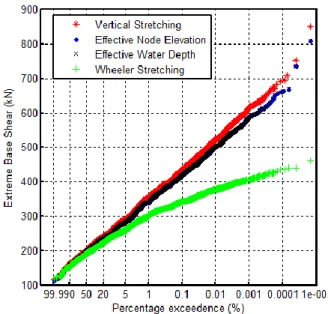
In this study, the Monte Carlo simulation technique has been used to derive the probability distributions of the extreme responses from the four different methods of simulating water particle kinematics based on 20000 simulated records, each of 128sec duration. 20000 simulated extreme values will ensure that the sampling variability is low and would allow any systematic difference between the two distributions to be observed without any ambiguity [22]. Each signal itself is short to reduce the computational effort for the Wheeler method as in this method the very efficient fast Fourier transforms (FFT) cannot be used for evaluation of water particle kinematics from a simulated surface elevation record. It should be noted that in this study the conclusions for both base shear and overturning moments are similar when comparing the results from different Hs values. Therefore, it would better to show a sample of results for both responses to indicate generality of the conclusions. As an example, the probability distributions of the extreme responses from the four methods for the quasi-static overturning moment with Hs = 15m are compared in Figure 3. A similar comparison for the case of quasi-static base shear with Hs = 5m is given in Figure 4. As observed, in all cases, the extreme quasi-static response calculated from the effective node elevation and the effective water depth are between those from the Wheeler (lowest) and the vertical stretching methods (highest). This is because water particle kinematics from the Wheeler stretching method are lower than those that those from the vertical stretching method.
In view of the general belief that the vertical stretching method can overpredict the responses, the effective water depth procedure seems to be more suitable for practical application. Overall, it can be concluded that the difference between 100-year predictions from the Wheeler and the vertical stretching are too large to be neglected and therefore, further investigation is necessary to resolve this problem.
Figure 3: Comparison of probability distributions of extreme values of quasi-static overturning moment from 4 different methods of simulating water particle kinematics, 20000 sample records, T = 128sec. Hs = 5m, Tz =
7.94sec.
Figure 4: Comparison of probability distributions of extreme values of quasi-static base shear from 4 different methods of simulating water particle kinematics, 20000 sample records, T = 128sec. Hs = 5m, Tz = 7.94sec.
8 CONCLUSIONS
Linear random wave theory (LRWT) is well known to lead to water particle kinematics with exaggerated high frequency components in the vicinity of MWL. To avoid this problem, modified versions of LRWT, such as Wheeler, vertical stretching, effective node elevation and effective water depth methods, are used to prevent this problem. Each of
these methods is intended to calculate sensible kinematics above the MWL, yet they have been found to differ from one another in their predictions.
Comparison between different methods make it clear that water particle kinematics from the effective water depth and effective node elevation methods in the near surface zone lie between those from the Wheeler and the vertical stretching methods. This is promising as there is some evidence that the water particle kinematics under crests are underestimated by the Wheeler method and that those from the vertical stretching method are somewhat exaggerated.
The current investigation shows that the probability distributions of extreme responses based on the Wheeler and the vertical stretching methods can be significantly different from each other, leading to uncertainty as to which method should be used in design. Further research is therefore required to resolve this issue.
It would be desirable to compare the results from these methods with high-quality laboratory and field data to observe how well they compare with measured data. Alternatively, they could be compared with water particle kinematics simulated from the more accurate Hybrid Wave Model.
ACKNOWLEDGEMENTS
This paper is financially supported by the Ministry of Higher Education (Malaysia) [Grant number: R.K130000.7840.4F583] and Universiti Teknologi Malaysia [Grant number: Q.K130000.2540.09H42] which is gratefully acknowledged.
REFERENCES
[1] Morison, J.R., O’Brien, M.P., Johnson, J.W. and Schaaf, S.A. (1950), “The force exerted by surface waves on pile”, ASMEPetroleum Transactions, Vol. 189, pp. 149-154.
[2] Wheeler, J.D. (1970), “Method for calculating forces produced by irregular waves”,
Journal of Petroleum Technology, Vol. 22, No 3, pp. 359-367.
[3] Rodenbusch, G. and Forristal, G.Z. (1986), “An empirical model for random directional wave kinematics near the free surface”, In: Proceedings of the 18th Offshore Technology Conference, pp. 137-146.
[4] Marshall, P.W. and Inglis, R.B. (1986), “Wave kinematics and force coefficients”, ASCE Structures Congress, New Orleans, Louisiana, USA.
[5] Couch, A.T. and Conte, J.P. (1997), “Field verification of linear and nonlinear Hybrid
wave models for offshore tower response prediction”, Journal of Offshore Mechanics
and Arctic Engineering, Vol. 119, pp. 158-165.
[6] Zhang, J., Chen, L., Ye, M. and Randall, R.E. (1996), “Hybrid wave model for
unidirectional irregular waves, Part I. Theory and numerical scheme”, Applied Ocean
Research, Vol. 18, pp. 77-92.
[7] Spell, C.A., Zhang, J. and Randall, R.E. (1996), “Hybrid wave model for unidirectional
irregular waves, Part II. Comparison with laboratory measurements”, Applied Ocean
Research, Vol. 18, pp. 93-10.
[8] Longridge, J.K., Randall, R.E. and Zhang, J. (1996), “Comparison of experimental
irregular water wave elevation and kinematic data with new hybrid wave model
[9] Donelan, M.A., Anctil, F. and Doering, J.C. (1992), “A simple method for calculating the velocity field beneath irregular waves”, Coastal Engineering, Vol. 16, pp. 399-424. [10] Najafian, G., Mohd Zaki, N.I. and Aqel G. (2009), “Simulation of water particle
kinematics in the near surface zone”, In: Proceedings of the ASME 28th International Conference on Ocean, Offshore and Arctic Engineering, Hawaii, USA, pp. 1-6.
[11] Mohd Zaki, N.I. and Najafian, G. (2010), “Derivation of water particle kinematics in the near surface zone by the effective water depth procedure”, In: Proceedings of the ASME 29th International Conference on Ocean, Offshore and Arctic Engineering, Shanghai, China, pp. 1-7.
[12] Pierson, W.J. and Moskowitz, L.J. (1964), “A proposed spectral form for fully-developed
wind seas based on the similarity theory of S.A. Kitaigorodskii”, Journal of Geophysical Research, Vol. 69, No 24, pp. 5181-5190.
[13] Sarpkaya, T. and Isaacson M., (1981), “Mechanics of Wave Forces on Offshore Structures”, Van Nostrand Reinhold, New York.
[14] Moe, G. and Verley, R.L.P. (1980), “Hydrodynamic damping of offshore structures in
waves and currents”, In: Proceedings of the Offshore Technology Conference, pp.37- 44. [15] Borgman, L.E. (1969), “Ocean wave simulation for engineering design”. ASCE Journal
of Waterways and Harbours Division, 95(WW4), pp. 557–83.
[16] Rice, S.O. (1944), “Mathematical analysis of random noise”, Bell System Technical
Journal, Vol. 23, pp. 282-332.
[17] Tucker, M.J., Carter D.J.T. and Challenor, P.G. (1984), “Numerical simulation of a random sea: a common error and its effect upon wave group statistics”, Applied Ocean Research, Vol. 6, pp. 118-122.
[18] Grigoriu, M. (1993), “On the spectral representation method in simulation”, Probabilistic Engineering Mechanics, Vol. 8, No. 2, pp. 75-90.
[19] Forristall G.Z., Irregular wave kinematics from a kinematic boundary condition fit (KBCF). 1985; 7:202-212.
[19] Morooka, C.K. and Yokoo, I.H. (1997), “Numerical simulation and spectral analysis of irregular sea waves”, International Journal of Offshore and Polar Engineering, Vol. 7, No. 3, pp. 189-196.
[21] Mohd Zaki, N.I., Abu Husain, M.K. and Najafian, G. (2014), “Extreme Structural
Response Values from Various Methods of Simulation Wave Kinematics”. Ships and Offshore Structures Journal, Vol. 10, pp. 1-10.
[22] Mohd Zaki, N.I., Abu Husain, M.K. and Najafian, G. (2013), “Comparison of Extreme
Offshore Structural Response from Two Alternative Stretching Techniques”. The Open Civil Engineering Journal, Vol. 7, pp. 273-281.