ISSN: 2068 - 3537, E – ISSN (online) 2069 – 9476, ISSN – L = 2068 – 3537 Year XX, No. 2, 2014, pp. 7-20
Evaluating the Impact of a New Product on the Sales of
other Products
J. A. Vasilev
Julian Andreev Vasilev Faculty of Informatics
Varna University of Economics, Bulgaria
Abstract
The purpose of this article is to evaluate the impact of a new product on the sales of other products. Launching a new product may lead to increase or decrease of sales in the products of the same group. Customers may continue buying standard products or they may be oriented to new products. New products may cause internal competition. Statistical methods are applied. Time series analysis is used. Transactional database of a confectionary factory is the main source of data. The time series analysis is carried in two datasets – quantities of sales of three products on a daily basis and on a monthly basis. The main methods used are time series analysis and regression analysis. The three time series (corresponding to the three products) are separated into two parts – before and after launching the new product. It is proved that the new product does not affect the sales of the two other products. The new product is well accepted and its sales increase together with the sales of the two other products.
Keywords: launching a new product, sales analysis, forecasting, time series analysis, SPSS, transactional sales database, data transformations, SQL
Introduction
with several independent variables and one independent variable (usually the quantity of future sales) gives a vague idea of what happens in real life. Usually regression analysis is applied to find a trend – the dependency of sales on time. It should be marked that all models have an error. The error shows that other factors influence sales, but they are not included in the model.
Launching a new product is a creative technique. New products are invented because the life of people changes. Some people die, other people are born, other people start working. The change of generations leads to an inevitable change in the portfolio of products. A new product may be well accepted by the market or it may be rejected. Sometimes the logistics curve (or logistics function) is used by marketing specialists to describe the lifecycle of a new product. Since the market is very sensitive to all changes there may be a slight difference between textbooks and business.
Forecasting of sales is widely discussed and described. The launch of a new product starts generating transactional data. Since the product is new, the transactional database does not contain enough historical data to predict sales. Moreover the real trend may not be noticed graphically. Seasonal decomposition could not be done.
Literature review
Conventional retail markets are known to be quite different from electronic markets. Ahluwalia et al. (2013) examine the effect on pricing in relation to proximity to a culturally and socially significant peak shopping day [7]. They study the effects of consumer’s product rating, product popularity, and featured product website rankings. This study is based on a real case study. Data are extracted from a B2C retailer. Some articles (Brent at al., 2014, Singh and Das, 2013) focus on salesperson turnover [2], [8]. Their study uses database collected from ten different firms. Discriminant analysis is used.
Sales analysis is often connected with analysis of seasonal variations. Andy et al. (2013) try to identify seasonal variations in store-level visitor grocery demand [1]. Store trading information is used. Spatial analysis is applied. The authors prove a significant degree of seasonality in terms of their revenue.
product innovation processes [4]. The author tests the relationship between innovation performance and business performance (sales and profitability).
Some authors (Rojas-Mendez and Rod, 2013) use face-to-face survey questionnaires to analyze sales of wine producers [5]. They compare two different instruments for assessing market orientation. Food supply chains and small producers in confectionary factories are studied by Ogelthorpe and Heron (2013). They try to identify the observable operational and supply chain barriers and constraints that occur in local food supply chains [3].
New products usually affect sales of other products. Mokhtar (2013) investigates the relationship between customer focus and new product performance [9]. Data are collected using mail questionnaire survey approach. The results revealed that customer focus has a statistically significant association with new product performance. Graner and Missler-Behr (2013) try to find key determinants of the successful adoption of new product development methods [6]. Their article adopts a structural equation modeling approach and analyzes the subject based on a large empirical sample of 410 product development projects.
Data preparation
For the sake of the analysis of the impact of a new product in a confectionary factory, transactional data for sales are used. The period is January 2011 until May 2013. The new product is croissant with chocolate, launched on 30 March 2012. The two other products are croissant with Turkish delight and croissant with marmalade (launched on 14 January 2011). We do not use questionnaires. We use transactional data to monitor sales. The transactional database consists of 332 000 records. The extraction of data starts with Query 1. The result of its execution is given in Table 1.
Table no.1. Extracting the first date of launching products
Code_item Name_item First Ofdate
The SQL code for getting the initial information is the following:
SELECT Sales_transactions.code_item, Items.name_item, First(Sales_transactions.date_doc) AS FirstOfdate_doc
FROM Items INNER JOIN Sales_transactions ON Items.code_item = Sales_transactions.code_item
GROUP BY Sales_transactions.code_item, Items.name_item HAVING (((Sales_transactions.code_item)=189)) OR (((Sales_transactions.code_item)=190)) OR
(((Sales_transactions.code_item)=191))
ORDER BY Sales_transactions.code_item,
First(Sales_transactions.date_doc);
Now we have three time series – for the sales of three products. We have to monitor sales of items 189 and 191 before and after 30 March 2012. The new product is 190. Since the data in the database consists of transactional data, we have to extract data by using select queries. We use only sold quantities. We do not use values of sales.
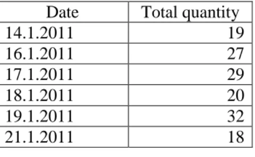
Table no.2. A part of the result dataset of “Total sales by dates for article number
Date Total quantity
14.1.2011 19
16.1.2011 27
17.1.2011 29
18.1.2011 20
19.1.2011 32
21.1.2011 18
The SQL code is the following:
SELECT Sales_transactions.[date_doc],
Sum(Sales_transactions.[quantity]) AS SumOfquantity FROM Sales_transactions
As it is obvious, the last SQL query gives a two dimensional dataset for sales. For those dates with zero sales no rows are added in the resulting dataset. So, some transformations in MS Excel may be made to fix this problem. By changing the string “189” to “190” and “191” we make two more select queries to extract time series for sales for items 190 and 191. But the problem with zero sales on some days exists. The result of the three queries is exported to MS Excel on a single worksheet. In a separate column all dates from 14 Jan 2011 until 5 May 2013 are filled automatically (844 days). By using the VLOOKUP function three new time series are created. They continue zero and non-zero values for sold quantities, for each date
We use three named ranges (SKU_189, SKU_190 and SKU_191). The first and the third data range consist of 819 rows and the second one, 396 rows. The formula for extracting zero and non-zero quantities is the following:
=IF(ISERROR(VLOOKUP(A3;SKU_189;2;FALSE));0;VLOOK UP(A3;SKU_189;2;FALSE))
Now the three new data series consist of 844 values – one value for each day. Each data series represents one stock keeping unit (SKU)
Table no. 3. A part of the three new data series
dates SKU 189
SKU 190
SKU 191
14.1.2011 19 0 14
15.1.2011 0 0 0
16.1.2011 27 0 14
17.1.2011 29 0 25
18.1.2011 20 0 19
19.1.2011 32 0 40
20.1.2011 0 0 0
Analyzing daily datasets in SPSS
The three data series contain numeric values. They may be exported from MS Excel and imported into SPSS [10]. Three variables are defined in SPSS – SKU_189, SKU_190 and SKU_191. All of them are on an interval scale. A string variable with dates is added in SPSS. It is recommended to use the natural logarithm function (ln) and seasonal decomposition before analyzing data series with time series analysis and building regression models. Our assumption is that a new product affects the sales of common products. The effect may be positive, the sales of two other products may increase or decrease or there may be no influence.
We have enough data to make the analysis. The period from 14.1.2011 until 6.5.2013 may be divided into two sub periods – before 30.3.2012 (the lunch of the new product) and after this date. We may use also case number (case numbers 1-441 are before launching the new product) to filter data series. Since we have a time series dataset, we have to define dates (Data/Define dates).
Three line charts may be made (before using the logarithmic function and seasonal decomposition) to see whether there is a trend in each time series.
Simple charts and values of individual cases are presented below.
It is obvious that there is a trend and sales of SKU 189 increase after case number 441.
Fig. no. 2. Line chart of SKU_191
It is obvious that there is a trend in SKU 191. Again the sales start to increase after case number 441. The graphs of SKU 181 and SKU 191 are almost the same.
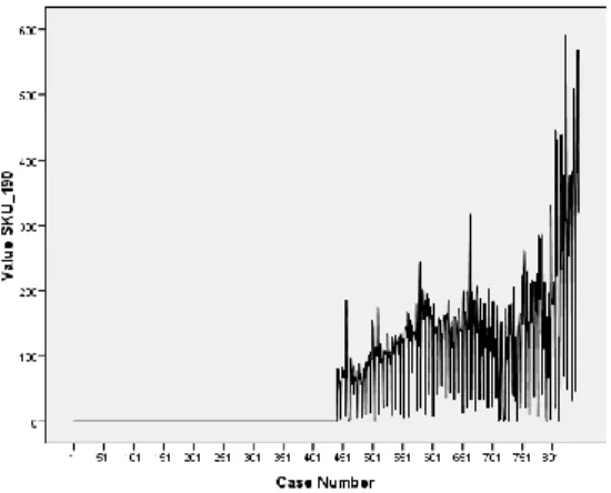
Fig. no. 3. Line chart of SKU_190 (the new product)
As a new product its sales are similar to the logistic function representing the launch of a new product.
The three time series seem to be correlated. It has to be checked for correlation. The check should be made for the two sub periods. First, we start with the first sub period (Data/Select Cases). We use selection of cases based on a satisfied condition (DAY_<=441). Then the existence of correlation is checked (Analyze/Correlate/Bivariate). Since the values in the three time series are in an interval scale, the Pearson correlation coefficient may be used. Two-tailed test of significance is made. The correlation between SKU 189 and SKU 191 is 0.915. The correlation is significant at 0.01 level (2-tailed).
Curve estimation may be made to check if the quantity of sales (of SKU 189 and SKU 191) depends on time (Analyze/Regression/Curve estimation). ANOVA tables are displayed. The constant is included in the equation. SPSS says that 17 cells have zero values so the compound, power, S, growth, exponential and logistic models cannot be calculated. All calculated models have R-square value less than 0.2. It means that it is almost impossible to create an equation which best represents the quantity of sales based on time for the first period.
The check for correlation between the three time series has to be made for the second sub period (cases > 441). Again a check for correlation is made. The correlation between SKU 189 and SKU 191 is 0.965 – even a higher value than the first sub period. The correlation between SKU 190 and SKU 189 is 0.949. The correlation between SKU 190 and SKU 191 is 0.974. The correlation coefficients are significant at 0.01 level (2-tailed). It means that when sold quantities of one of the three products increase, there is a great possibility the sales of the two other products two increase. Again curve estimation may be made for the three time series for the second sub period. ANOVA tables are displayed. The constant is included in the equation. The highest R-square value is for the cubic function (0.331) but it is not very high to make a meaningful equation. By excluding the constant in equation the highest value of R-square has the cubic function (0.812).
automatically calculated – lnSKU_189, lnSKU_190 and lnSKU_191. Seasonal decomposition is made (Analyze/Forecasting/Seasonal Decomposition). Since we have very detailed data (for daily sales) SPSS says “Seasonal decomposition requires at least one periodic data component to be defined”. If we aggregate data on a monthly basis we will not get this error but we will lose a lot of detailed information. The dispersion in the three initial series is stabilized by calculating the natural logarithm.
A check for autocorrelation has to be made for each time series (Analyze/Forecasting/Autocorrelations). For the three time series (lnSKU_189, lnSKU_190 and lnSKU_191) the partial autocorrelation coefficients (ACF) are outside the upper and the lower confidence limit. It means that there is autocorrelation in the three time series. We have to create a time series by using the first order of the difference function for the three time series lnSKU_189, lnSKU_190 and lnSKU_191 (Transform/Create time series).
Three new time series are created: lnSKU__189, lnSKU__190 and lnSKU__191. Again a check for autocorrelation is made. The partial ACF are again outside the lower and upper confidence limit. So the conclusion is that a mathematical formula for calculating future sales cannot be made. Moreover linear regression for SKU_189 and SKU_191 cannot be done neither for the first, nor for the second sub period. Thus a calculation for the influence of the new product 190 cannot be calculated. Even though sales of the three products are increasing during the second sub period it may not be proved that the increase of sales is caused by launching a new product.
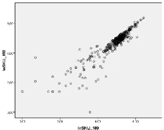
Fig. no. 4. Dependency between lnSKU_189 and lnSKU_190
By using curve estimation the linear model may be checked. The independent variable is lnSKU_189 and the dependent variable is lnSKU_190. The R-square value is 0.814. The ANOVA test shows that the model is adequate. The unstandardized coefficient B is 0.903. It is statistically significant. The constant in the equation is 0.274. It is statistically not significant. So the conclusion is that we may do the curve estimation by excluding the constant in equation. Now the R-square value is 0.993. The ANOVA test shows that the model is adequate. The unstandardized coefficient B is 0.957. It is statistically significant. The equation is the following:
Ln( Y ) = 0.957 * Ln( X )
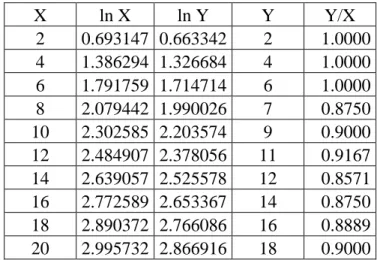
Table no. 4. Predicted quantities for SKU 190 (variable Y) on the basis of sold quantities for SKU 189 (variable X)
X ln X ln Y Y Y/X
2 0.693147 0.663342 2 1.0000 4 1.386294 1.326684 4 1.0000 6 1.791759 1.714714 6 1.0000 8 2.079442 1.990026 7 0.8750 10 2.302585 2.203574 9 0.9000 12 2.484907 2.378056 11 0.9167 14 2.639057 2.525578 12 0.8571 16 2.772589 2.653367 14 0.8750 18 2.890372 2.766086 16 0.8889 20 2.995732 2.866916 18 0.9000
The top left corner of the table is situated in C2. The formula for calculating ln X is: “= ln (C3)”. The formula for ln Y is “=D3*0.957”. The formula in Y column is “=ROUND(EXP(1)^E3;0)”. The last column “Y/X” is “=F3/C3”. The last column calculates the slope of the line.
Analyzing monthly datasets in SPSS
Using daily datasets we proved that we could not make regression analysis. By grouping the initial three datasets on a monthly basis, similar calculations may be made. Our prediction is the same. The trend line of sales of SKU 189 changes when launching the new product 190. We will skip the dataset for SKU 191, because we calculated a great correlation between SKU 189 and SKU 191.
Aggregating time series may be done in MS Excel or directly with a SQL query. We will use the first approach. Firstly, we copy the first three columns from table 3 on a separate worksheet. By using the built-in functions “month” and “year”, the month and year of each date is extracted. Data are grouped by a Pivot table. “Year” and “month” are used for row labels. “Sum of SKU 189” and “Sum of SKU 190” are used as summary values.
we use the total sold quantity of each product for each month. We lost a lot of data but we may make seasonal decomposition and try to make regression analysis for the two periods for SKU 189.
In SPSS we define four variables on an interval scale – year, month, SKU_189 and SKU_190. Dates are defined. Cases are years and months starting from year: 2011 and month: 1. Natural logarithm of both time series is calculated. Seasonal decomposition has to be done. The additive model is used. Seasonal decomposition cannot be done because of missing data for SKU 190 – it is a new product. Seasonal decomposition cannot be done for SKU 189 because at least four full seasons of data must exist.
Now three linear models for SKU 189 have to be tested – for the whole period, before and after launching the new product. The models may be only linear, because we used the logarithmic function.
The first model (for the whole period) including the constant in equation is checked. The R-square value is 0.703. The ANOVA test shows that the model is adequate. The unstandardized coefficient B value is 0.069, the constant is 6.775. Both coefficients are statistically significant. By excluding the constant in equation the R-square value is 0.821. The ANOVA test shows that the model is adequate. The unstandardized coefficient B value is 0.414. It is statistically significant. For the whole period we have increasing sales. The slope of the line is 0.414.
The second model (before launching the new product) including the constant in equation is checked. The R-square value is 0.542. It is comparatively low. The model and the calculated coefficients are significant at Alfa 0.05. Not including the constant in equation the R-square value is 0.813. The model is adequate. The slope of the line is 0.771.
The third model (after launching the product) with constant in equation has a very low value of R-square 0.126. Excluding the constant in equation the R-square value is 0.787. The unstandardized coefficient B (the slope of the line showing the natural logarithm of sales) is 0.813. It is statistically significant.
Conclusions
Confectionary factories have a lot of data stored in a transactional database. Transactional databases are mainly used to record sales and organize the logistics activity. In rear cases they may be used for data mining. Launching a new product may cause serious fluctuations in the sales of other products from the same group. In this study three products are monitored. Two of them are sold 844 days. The third one goes out to market on the 441 day. The initial prediction is that the new product affects the sales of the two other products. It is calculated that there is a strong correlation between the three products. As a whole (during the whole period) the sales of the three products increase. The period of 844 days is divided into two parts – before launching the new product and after launching the product. The time series of one of the products is analyzed, because there is a strong correlation between the sales of the three products. Three linear models are estimated – for the whole period, before launching the new product and after launching it. It is proved that the new product does not affect the sales of the two other products. Time series analysis is used. Regression analysis is not applied at its final stage, because of a strong autocorrelation in the three time series. Autocorrelation cannot be removed by standard statistical methods. Future research may focus on extended models where other independent variables are included.
References
[1] Newing, A., Clarke, G., Clarke, M. (2013). Identifying seasonal variations in store-level visitor grocery demand, International Journal of Retail & Distribution Management, Vol. 41 Issue: 6, p. 477 – 492.
[2] Wren, B. M., Berkowitz, D., Grant, E. S. (2014). Attitudinal, personal and job-related predictors of salesperson turnover, Marketing Intelligence & Planning, Vol. 32 Issue: 1, p.107 – 123.
[4] Löfsten, H. (2014). Product innovation processes and the trade-off between product innovation performance and business performance, European Journal of Innovation Management, Vol. 17 Issue: 1, p. 61 – 84.
[5] Rojas-Méndez, J. I., Rod, M. (2013). Chilean wine producer market orientation: comparing MKTOR versus MARKOR, International Journal of Wine Business Research, Vol. 25 Issue: 1, p. 27 – 49
[6] Graner, M., Mißler-Behr, M. (2013). Key determinants of the successful adoption of new product development methods, European Journal of Innovation Management, Vol. 16 Issue: 3, p. 301 – 316
[7] Punit, A., Hughes, J., Midha, V. (2013). Drivers of e-retailer peak sales period price behavior: an empirical analysis, International Journal of Accounting and Information Management, Vol. 21 Issue: 1, p. 72 – 90.
[8] Singh, R., Das, G. (2013). The impact of job satisfaction, adaptive selling behaviors and customer orientation on salesperson's performance: exploring the moderating role of selling experience, Journal of Business & Industrial Marketing, Vol. 28 Issue: 7, p. 554 – 564.
[9] Mohd Mokhtar, S. S. (2013). The effects of customer focus on new product performance, Business Strategy Series, Vol. 14 Issue: 2/3, p. 67 – 71.