Nonparametric Bounds for the Risk Function
Stephen R. Cole*, Michael G. Hudgens, Jessie K. Edwards, M. Alan Brookhart, David B. Richardson, Daniel Westreich, and Adaora A. Adimora
*Correspondence to Dr. Stephen R. Cole, Department of Epidemiology, Gillings School of Global Public Health, UNC Campus Box 7435, Chapel Hill, NC 27599-7435 (e-mail: [email protected]).
Initially submitted May 31, 2018; accepted for publication January 11, 2019.
Nonparametric bounds for the risk difference are straightforward to calculate and make no untestable assump-tions about unmeasured confounding or selection bias due to missing data (e.g., dropout). These bounds are often wide and communicate uncertainty due to possible systemic errors. An illustrative example is provided.
bias; bounds; inference; missing data
Abbreviation: AIDS, acquired immune deficiency virus.
Nonparametric bounds are the minimum and maximum val-ues of the target parameter (e.g., risk difference) that are com-patible with the observed data (1–3). We are often interested in bounds because, assuming we believe the observed data, these bounds provide the space in which the true but unknown parame-ter value must lie. The difference in the risk of an outcome if everyone in the population were treated minus the same risk if everyone were untreated is a causal risk difference, which has a possible range from−1 to 1 (4). In contrast, the associational risk difference is the difference in the risk of an outcome for those observed to be treated minus the same risk for those observed to be untreated. In observational data, the associational risk differ-ence is point-identified (i.e., we can compute a single numerical value), but the causal risk difference is not identified without additional untestable assumptions. The causal risk difference is point-identified when treatment is assigned randomly, as in ran-domized experiments.
It is commonly believed that bounds on the causal risk dif-ference (henceforth, “risk difference”) for nonrandomized data are uninformative. The logic for this belief is based on the observation that such bounds are guaranteed to have unit length and thereby always include the null hypothesis value of a zero risk difference (1). We believe this is a pessimistic perspective.
An optimist might say that such bounds cut the interval for the possible range of the risk difference in half. The bounds do so with identification conditions stemming from causal consis-tency (5–7) and negligible measurement bias (8) and
notably do not require exchangeability of treated and untreated groups (i.e., unmeasured confounding might be present). Bounds properly reveal an ignorance interval associated with a possible lack of exchangeability that occurs in the absence of randomiza-tion (9). In expectation, ideal randomized experiments guarantee exchangeability between treatment groups by design. In such cases, the upper and lower bounds collapse to the same point.
With an important exception (1), discussions and illustrations of nonparametric bounds are typically limited to a single proba-bility (2,3,10–13) rather than the set of probabilities that define a survival or risk function (14). In making such a simplification, discussions fail to address the possible uncertainty due to selec-tion bias from missing data, such as censoring due to dropout, which affects both randomized and nonrandomized studies (15). Here we illustrate how to estimate nonparametric bounds on the risk difference function over time, which accounts for possible unmeasured confounding as well as selection bias due to missing data.
METHODS
Example data
baseline use of injection drugs, as well as the risk difference, over the 10-year follow-up period. We note that injection drug use in these data is prevalent at baseline, and use might change over follow-up. For pedagogical purposes, we imagine that drug use is incident andfixed over follow-up (alternatively, we wish to learn the effect of the point exposure of drug-use initiation). Specifically, we estimate the crude risk difference function and the bounds for the risk difference function.
Women were followed from December 6, 1995 (baseline), for a combined outcome of incident AIDS diagnosis or death from any cause. Of 1,164 women, 439 (38%) were classified as exposed to injection drug use based on data reported as of base-line; 672 of 1,164 women (58%) were black. The median age was 36 (quartiles: 31, 41) years at baseline, and lowest recorded CD4 count prior to baseline was 139 (quartiles: 85, 207) cells/ mm3. Of the 1,164 women, 127 (11%) were lost to follow up.
Statistical methods
We assume throughout that the sample of women is effec-tively a random sample from the population of interest, such that we can ignore the issue of generalizability (19). We assume that the data are measured with negligible error (20), that there is no interference (21), and that exposure versions are irrelevant (5,6). For all estimates, we present pointwise 95% confidence intervals based on a standard asymptotic nor-mal approximation of the crude and bounded risk differences (i.e., bˆ −L 1.96×se b( ˆ )L tobˆ +U 1.96×se b( ˆ )U , where bˆL
andbUˆ are the estimated lower and upper bounds). These
con-fidence intervals coincide with what Vansteelandt et al. (9) call a strong uncertainty region. Next we describe the bounds.
First, assume complete follow-up data for all subjects (i.e., no dropout). Treatment (or exposure) is denoted asA= a, saya= {0, 1}. Suppose the outcome of interest is an event time, denoted asT, whereT>0. Letτ denote the maximum follow-up length (here τ =10 years). Let T a( ) denote the potential outcome (or counterfactual) event time under treatment
=
A a. Then, by the law of total probability, the counterfactual risk at timetfora=1,P T{ ( ) < }1 t , equals
{ ( ) < | = } ( = )
+ { ( ) < | = } ( = ) ( )
P T t A P A
P T t A P A
1 0 0
1 1 1 1
Likewise for a=0. We observe treatment A and event time T, but we do not observe both counterfactuals T( )0,
( )
T 1. The second probability in equation1is the complement of the fourth probability, both of which are identified with observed data. With a sample ofnsubjects, we may consis-tently estimateP A( = )a using the nonparametric estimator
ˆ ( = ) = − ∑ ( = )
=
P A a n 1 in 1 I Ai a. Under causal consistency,
the third probability in equation1is also identified, and we may consistently estimate it similarly. In a nonrandomized study, thefirst probability in equation1is not identified with-out additional assumptions (e.g., exchangeability), and there-fore cannot have a consistent estimator. However, the first probability may be replaced with its bounds of 0 and 1 to pro-vide bounds for the counterfactual risksP T a{ ( ) < }t . Note that the unidentifiedfirst probability in equation1is scaled by the probability of being untreated P A( = )0, such that the bounds onP T{ ( ) < }1 t (or treated risk bounds) are a func-tion of the proporfunc-tion untreated (e.g., if 2/3 are treated, then the bounds for the treated risk have width 1/3). Likewise, for the untreated risk bounds. Therefore, when we take the maxi-mal difference between the treated risk bounds and the untreated risk bounds, we have a resulting unit length.
Next letΔ =1indicate an observed study event, and sup-pose a fraction of subjects are missing data on their event time
T (e.g., due to dropout), in which case,Δ =0. The target parameter remainsP T a{ ( ) < }t and can now be expressed as
δ δ
∑δ,aP T a{ ( ) < |Δ =t ,A= } (Δ =a P ,A= )a.
Identi-fied probabilities can be consistently estimated using nonparametric estimators, and unidentified probabilities can be replaced with bounding values, both as above. Bounds that account for both confounding and selection bias will be wider than unit interval.
All that remains is to calculate the bounds. We can opera-tionalize the above approach as follows. For each subject, create a doppelganger (or copy) with the treatment set to its complement. For thefirst of 2 bounds, treated doppelgangers
Table 1. Ten-Year Risks of Diagnosis of Acquired Immune Deficiency Syndrome or Death From Any Cause According to Injection Drug Use in the Women’s Interagency HIV Study, United States, 1995–2006
Approach No. of Participants No. of AIDS Diagnoses or Deaths 10-Year Risk 10-Year Risk Difference 95% CI
Crude
Injection drug use 439 272 64.0 18.5 12.5, 24.5
Nonuse 725 307 45.5 0
IP-weighteda
Injection drug use 439 272 63.0 16.0 10.0, 22.1
Nonuse 725 307 47.0 0
Bounded
Injection drug use 439 272 and 1,023b 23.4 and 87.9b −49.4 to 61.5 −52.3, 64.3
Nonuse 725 847 and 307b 72.7 and 26.4b 0
Abbreviations: AIDS, acquired immune deficiency syndrome; CI, confidence interval; HIV, human immunodeficiency virus; IP, inverse probability.
are immediate events atT= ϵ(whereϵ >0is smaller than thefirst observed event time), and untreated doppelgangers are nonevents at the end of the study periodT= τ. Con-versely, for the second of 2 bounds, treated doppelgangers are nonevents at the end of the study period and untreated doppelgangers are immediate events.
To further account for possible selection bias due to missing data (e.g., dropout), the observed data from nondoppelgangers is altered as follows. For thefirst of 2 bounds, treated observa-tions with unobserved eventsΔ =0are set to be events at the time last observed T=t, and untreated observations with unobserved eventsΔ =0 are set to remain nonevents with times moved to the end of the study periodT= τ. For the sec-ond of 2 bounds the converse is undertaken. Of course, one can estimate bounds selectively accounting for possible selection bias due to missing data, while assuming treatment groups are exchangeable (i.e., no confounding), as might occur in a ran-domized experiment. Illustrative pseudocode is presented in the
Appendix.
RESULTS
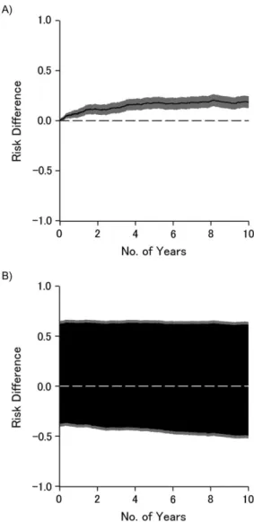
Table1presents estimates of the 10-year risks of AIDS diag-nosis or death from any cause according to injection drug use. As can be seen, accounting for measured confounders age, race, and nadir CD4 using inverse-probability weighting did not mate-rially alter the 10-year risks or risk difference, compared with the crude risks and risk difference. The 10-year bounded risk differ-ence was, as expected, notably wide compared with the point estimator, which assumes no confounding or selection bias. Figure1illustrates the crude risk difference (Figure1A) and the risk difference bounded for confounding and selection bias (Figure1B) as functions of time on study; the black lines (or areas) represent point (or set) estimates, and gray areas repre-sent the 95% confidence intervals. Briefly, the effect apparent under the strong assumption of no unmeasured confounding or selection bias weakens to become only suggestive once we allow for possible unmeasured confounding and selection bias. Other investigators provide detailed systematic exploration of how to leverage information provided in the bounds (1,12,22).
DISCUSSION
What would it mean to solve the problem of unmeasured con-founding? Of course, the problem of unmeasured confounding is solved already in the sense that randomized experiments provide point-identified solutions for effects of treatment assignment (23). Randomized experiments prevent unmeasured confounding; at least the ideal experiment does so in expectation. Rather, when try-ing to“solve the problem of unmeasured confounding,”we often mean not prevention but cure. How do we cure the problem of unmeasured confounding in nonrandomized studies? It is helpful to think about how we would do so in a randomized experiment that was broken in the sense that key data were missing. Any such prevention or cure would avoid (or at least weaken) an assumption of no unmeasured confounding, as does the randomized experi-ment. Such exchangeability assumptions (e.g., no unmeasured confounding, appropriate instrumental variable (24)) are the current state of the science in nonrandomized studies. Perhaps a
cure would yield point-identified answers, akin to randomized experiments. Perhaps it would be folly to expect point identifi -cation without randomization or something nearly as strong.
However as soon as we relax our insistence on point iden-tification, we have a solution in hand, albeit not widely rec-ognized. The solution does not require any assumption about unmeasured confounding, and the solution immediately and simply allows estimates as well as confidence intervals. The solution is to provide an interval or set estimate, rather than a point estimate. Simply put, bounds are a solution to the prob-lem of unmeasured confounding. Recalling Tukey’s apocry-phal use of out-of-focus slides to convey uncertainty, in the presence of uncertainty about confounding, we have to draw ourfigures with a thick marker instead of a sharp pencil.
region is a conservative pointwise uncertainty interval for the parameter of interest, and tighter intervals with appropriate coverage can be obtained by replacing the standard multiplier by an alternative described in Vansteelandt et al. (9) and Imbens and Manski (25). For bounds that include minimum or maxi-mum functions, such as instrumental variable bounds (26), alternative inferential methods are needed to construct valid confidence intervals (27). Here we discussed pointwise uncer-tainty intervals for the bounds of the risk functions; one could also entertain simultaneous uncertainty bands for the bounds of the risk function, analogous to the well-known distinction for confidence bands (28, p. 109). In some settings the width of the bounds might also be reduced by using covariates that are associated with treatment or the outcome (29).
The foremost argument against the use of bounds is that they are uninformative. That the bounds are often uninforma-tive is itself highly informauninforma-tive: It is usually good to learn what one does not know! Such bounds provide a frame of reference in which the actual treatment or exposure effect lies (to the extent that data are measured without error). Such bounds also provide a logical underpinning to further refi ne-ments on analyses, such as point identification by assuming no unmeasured confounding as well as providing a space for sensitivity analyses to span. However, presenting the bounds alongside traditional point estimates provides helpful context in settings where nonrandomized data are the only feasible route to causal inference. In some settings, particularly those with either strong prior beliefs or strong preference functions, policy decisions can be grounded on set-identified bounding analyses (22).
We are not thefirst to call for presentation of bounds. For example, Swanson et al. conclude“If nothing else, estimating the bounds can serve as a reminder to remain humble about how much information the data really provide”(26, p. 945). Robins and Greenland argue for reporting bounds and state
“Wide bounds make clear the degree to which public health decisions are dependent on merging the data with strong prior beliefs”(30, p. 457). Finally, perhaps such bounds will pro-vide a bridge over which those conducting observational stud-ies can communicate with colleagues conducting clinical trials with more signal and less noise.
(Gillings Innovation Laboratory award to S.R.C., M.G.H., J. K.E., and D.W.) and by the National Institutes of Health (grants R01AI100654 to S.R.C., M.G.H., and D.W.; R24AI067039 to S.R.C.; U01AI103390 to A.A.A., S.R.C., and D.W.; DP2HD084070 to D.W. and S.R.C.;
K01AI125087 to J.K.E.; and P30AI50410 to M.G.H. and S.R.C.).
We thank Drs. Alexander Breskin, Ashley I. Naimi, and Robert W. Platt for expert advice.
Conflict of interest: none declared.
REFERENCES
1. Robins JM. The analysis of randomized and nonrandomized AIDS treatment trials using a new approach to causal inference in longitudinal studies. In: Sechrest L, Freeman H, Mulley A, eds.Health Service Research Methodology: A Focus on AIDS. Washington, DC: US Public Health Service; 1989:113–15959. 2. Manski CF. Nonparametric bounds on treatment effects.Am
Econ Rev. 1990;80(2):319–323.
3. Balke A, Pearl J. Bounds on treatment effects from studies with imperfect compliance.J Am Stat Assoc. 1997;92(439): 1171–1176.
4. Robins JM. Confidence intervals for causal parameters.Stat Med. 1988;7(7):773–785.
5. Cole SR, Frangakis CE. The consistency statement in causal inference: a definition or an assumption?Epidemiology. 2009; 20(1):3–5.
6. VanderWeele TJ. Concerning the consistency assumption in causal inference.Epidemiology. 2009;20(6):880–883. 7. Pearl J. On the consistency rule in causal inference: axiom,
definition, assumption, or theorem?Epidemiology. 2010;21(6): 872–875.
8. Hernán MA, Cole SR. Invited commentary: causal diagrams and measurement bias.Am J Epidemiol. 2009;170(8):959–962. 9. Vansteelandt S, Goetghebeur E, Kenward MG, et al. Ignorance
and uncertainty regions as inferential tools in a senstivity analysis.Stat Sin. 2006;16:953–979.
10. Balke A, Pearl J. Counterfactual probabilities: computational methods, bounds, and applications. In: Lopez de Mantara R, Poole D, eds.Uncertainty in Artifical Intelligence. San Mateo, CA: Morgan Kaufman; 1994:46–54.
11. Cole SR, Hudgens MG, Edwards JK. A fundamental equivalence between randomized experiments and
observational studies.Epidemiol Methods. 2016;5(1):113–117. 12. Swanson SA, Holme Ø, Loberg M, et al. Bounding the
per-protocol effect in randomized trials: an application to colorectal cancer screening.Trials. 2015;16:541.
13. Pearl J.Causality. 2nd ed. New York, NY: Cambridge University Press; 2009.
14. Cole SR, Hudgens MG, Brookhart MA, et al. Risk.Am J Epidemiol. 2015;181(4):246–250.
15. Little RJ, D’Agostino R, Cohen ML, et al. The prevention and treatment of missing data in clinical trials.N Engl J Med. 2012; 367(14):1355–1360.
16. Lau B, Cole SR, Gange SJ. Competing risk regression models for epidemiologic data.Am J Epidemiol. 2009;170(2): 244–256.
17. Barkan SE, Melnick SL, Preston-Martin S, et al. The Women’s Interagency HIV Study.Epidemiology. 1998;9(2):117–125. 18. Adimora AA, Ramirez C, Benning L, et al. Cohort profile: the
Women’s Interagency HIV Study (WIHS).Int J Epidemiol. 2018;47(2):393–394i.
ACKNOWLEDGMENTS
Authoraffiliations:DepartmentofEpidemiology,Gillings SchoolofGlobalPublicHealth,UniversityofNorth
Carolina,ChapelHill,NorthCarolina(StephenR.Cole, JessieK.Edwards,M.AlanBrookhart,DavidB. Richardson,DanielWestreich,AdaoraA.Adimora); DepartmentofBiostatistics,GillingsSchoolofGlobal PublicHealth,UniversityofNorthCarolina,ChapelHill, NorthCarolina(MichaelG.Hudgens);NoviSciLLC, Durham,NorthCarolina(M.AlanBrookhart);and
DepartmentofMedicine,SchoolofMedicine,Universityof NorthCarolina,ChapelHill,NorthCarolina(AdaoraA. Adimora).
19. Lesko CR, Buchanan AL, Westreich D, et al. Generalizing study results: a potential outcomes perspective.Epidemiology. 2017;28(4):553–561.
20. Edwards JK, Cole SR, Westreich D. All your data are always missing: incorporating bias due to measurement error into the potential outcomes framework.Int J Epidemiol. 2015;44(4): 1452–1459.
21. Hudgens MG, Halloran ME. Toward causal inference with interference.J Am Stat Assoc. 2008;103(482):832–842. 22. Manski CF.Public Policy in an Uncertain World: Analysis and
Decisions. Cambridge, MA: Harvard University Press; 2013. 23. Fisher RA. The arrangement offield experiments.J Minist
Agric Great Britain. 1926;33:503–513.
24. Greenland S. An introduction to instrumental variables for epidemiologists.Int J Epidemiol. 2000;29(4):722–729. 25. Imbens GW, Manski CF. Confidence intervals for partially
identified parameters.Econometrica. 2004;72(6):1845–1857. 26. Swanson SA, Hernán MA, Miller M, et al. Partial identification
of the average treatment effect using instrumental variables: review of methods for binary instruments, treatments, and outcomes.J Am Stat Assoc. 2018;113(522):933–947. 27. Tamer E. Partial identification in econometrics.Annu Rev
Econ. 2010;2:167–195.
28. Klein JP, Moeschberger ML.Survival Analysis: Techniques for Censored and Truncated Data. 2nd ed. New York, NY: Springer; 2003.
29. Lee DS. Training, wages, and sample selection: estimating sharp bounds on treatment effects.Rev Econ Stud. 2009;76(3): 1071–1102.
30. Robins JM, Greenland S. Comment on Angrist, Imbens and Rubin: estimation of the global average treatment effects using instrumental variables.J Am Stat Assoc. 1996;91:456–458.
APPENDIX
Algorithm to calculate bounds
Bound algorithm:
1. Bound 1, the worst case for treated. 2. Alter the observed record.
Ifa=1 andΔ=0 then:a1=a,Δ1=1,t1=t. Else ifa=0 andΔ=0 then:a1=a,Δ1=0,t1=τ. Else ifΔ=1 then:a1=a,Δ1=Δ,t1=t.
3. Augment data with a doppelganger. Ifa=1 then:a1=1–a,Δ1=0,t1=τ. Else ifa=0 then:a1=1–a,Δ1=1,t1=ε.
4. Adapt above steps for bound 2, the worst case for untreated.
5. Compute standard estimators for risk to the altered and augmented data.