Cui_unc_0153D_17589.pdf

TREE-BASED SURVIVAL MODELS AND PRECISION MEDICINE

Yifan Cui

A dissertation submitted to the faculty of the University of North Carolina at

Chapel Hill in partial fulfillment of the requirements for the degree of Doctor of

Philosophy in the Department of Statistics and Operations Research.

Chapel Hill

2018

Approved by:

Shankar Bhamidi

Jan Hannig

c

2018

Yifan Cui

ABSTRACT

YIFAN CUI: Tree-based survival models and precision medicine

(Under the direction of Dr. Michael R. Kosorok and Dr. Jan Hannig)

Random forests have become one of the most popular machine learning tools in recent years.

The main advantage of tree- and forest-based models is their nonparametric nature. My dissertation

mainly focuses on a particular type of tree and forest model, in which the outcomes are right censored

survival data. Censored survival data are frequently seen in biomedical studies when the true clinical

outcome may not be directly observable due to early dropout or other reasons.

We first carry out a comprehensive analysis of survival random forest and tree models and

show the consistency of these popular machine learning models by developing a general theoretical

framework. Our results significantly improve the current understanding of such models and this is

the first consistency result of tree- and forest-based regression estimator for censored outcomes under

high-dimensional settings. In particular, the consistency results are derived through analyzing the

splitting rules and establishing an adaptive concentration bound of the variance component, which

may also shed light on the theoretical analysis of other random forest models.

In the second part, motivated by tree-based survival models, we propose a fiducial approach to

provide pointwise and curvewise confidence intervals for the survival functions. On each terminal

node, the estimation is essentially a small sample and maybe heavy censoring problem. Most of the

asymptotic methods of estimating confidence intervals have coverage problems in many scenarios.

The proposed fiducial based pointwise confidence intervals maintain coverage in these situations.

Furthermore, the average length of the proposed pointwise confidence intervals is often shorter than

the length of competing methods that maintain coverage.

I dedicate this dissertation work to my parents,

Chaojie Cui and Hong Ruan,

and my grandparents,

Zhentian Ruan and Shihua Zhang,

ACKNOWLEDGEMENTS

I am very grateful to all of those who contributed in some way to the work in this thesis.

First and foremost, my deepest gratitude is to my advisors, Dr. Michael R. Kosorok and Dr. Jan

Hannig, for their enthusiasm, guidance, encouragement, and support. Their mentoring has been

both inspirational and cheered me during my venture. I have been extremely lucky to have two

advisors who cared so much about my work, and lent invaluable assistance to my study and research.

It is much more than statistics that I learned from them. I would not have been able to achieve

this accomplishment without them. I would also like to thank Dr. Kosorok for providing me the

opportunity to visit the University of Cambridge to conduct research on adaptive clinical trials.

I would also like to thank my committee members Professor Shankar Bhamidi, Donglin Zeng,

and Kai Zhang for reading the manuscript and offering insightful comments which have led to

significant improvements of the thesis.

I would like to thank Dr. Ruoqing Zhu, Dr. Mai Zhou, and Dr. Stefan Wager. My collaboration

with them has been a very enjoyable part of my graduate study.

I am also thankful to all other faulty members, students and staff in the Department of Statistics

and Operations Research and Department of Biostatistics.

My sincere thanks also go to Dr. James Hung, Dr. Peiling Yang, and Dr. Semhar Ogbagaber,

for offering me the summer research opportunities at the Food and Drug Administration and leading

me to work on sequential parallel comparison designs.

TABLE OF CONTENTS

LIST OF TABLES . . . .

x

LIST OF FIGURES . . . .

xi

1

Introduction . . . .

1

1.1

Some asymptotic results for survival tree and forest models . . . .

1

1.2

Nonparametric generalized fiducial inference for survival functions under censoring . . .

1

1.3

Tree based weighted learning for estimating ITRs with censored data . . . .

2

2

Some asymptotic results for survival tree and forest models . . . .

3

2.1

Introduction . . . .

3

2.2

Tree-based survival models . . . .

4

2.3

The splitting rule and its biasedness . . . .

6

2.3.1

Within-node estimation . . . .

7

2.3.2

A motivating example . . . .

8

2.3.3

Survival estimation based on independent but non-identically

dis-tributed observations . . . .

9

2.4

Adaptive concentration bounds of survival trees and forests . . . 12

2.4.1

Additional definitions . . . 12

2.4.2

Main result . . . 14

2.5

Consistency of survival tree and forest models . . . 16

2.5.1

Consistency of survival forest when dimension

d

is fixed . . . 17

2.5.2

Consistency of survival forests with a nonparametric splitting rule

when dimension

d

is infinite . . . 18

2.6

Discussion . . . 21

3.1

Introduction . . . 23

3.2

Methodology . . . 25

3.2.1

Fiducial approach explained . . . 25

3.2.2

Fiducial approach in survival setting . . . 28

3.2.3

Inference based on fiducial distribution . . . 31

3.3

Theoretical results . . . 34

3.4

Simulation study . . . 37

3.4.1

Coverage of pointwise confidence intervals and mean square error of

point estimators . . . 37

3.4.2

Comparisons between the proposed fiducial test and different types

of log-rank tests for two sample testing . . . 41

3.5

Gastric tumor study . . . 44

3.6

Discussion . . . 45

4

Tree based weighted learning for estimating ITRs with censored data . . . 47

4.1

Introduction . . . 47

4.2

Methodology . . . 48

4.2.1

Individualized treatment regime framework . . . 48

4.2.2

Value function under right censoring . . . 50

4.2.3

Outcome weighted learning with survival trees . . . 51

4.3

Theoretical results . . . 53

4.3.1

Preliminaries . . . 53

4.3.2

Consistency of tree-based survival models . . . 53

4.3.3

Consistency and excess value bound . . . 55

4.4

Simulation studies . . . 57

4.4.1

Simulation settings . . . 58

4.4.2

Simulation results . . . 60

4.5

Data analysis . . . 62

Appendix A: Supplementary material to Chapter 2 . . . 66

Appendix B: Supplementary material to Chapter 3 . . . 83

Appendix C: Supplementary material to Chapter 4 . . . 93

LIST OF TABLES

2.1

Probability of selecting the splitting variable. . . .

9

3.1

Error rate (in percent) and average width of

95%

confidence intervals for

scenario 1 . . . 40

3.2

Error rate (in percent) and average width of

95%

confidence intervals for

scenario 2 . . . 40

3.3

Mean square error of survival function estimators . . . 40

3.4

Percentage of p-value less than 0·05 (

%

) for scenario 1 . . . 43

3.5

Percentage of p-value less than 0·05 (

%

) for scenario 2 . . . 43

3.6

Percentage of p-value less than 0·05 (

%

) for scenario 3 . . . 43

3.7

Percentage of p-value less than 0·05 (

%

) for scenario 4 . . . 44

3.8

Gastric tumor study: p-value of different tests (in %) . . . 44

3.9

Gastric tumor study: Percentage of p-value less than 0·05 (

%

) . . . 45

4.1

Simulation results: Mean and standard deviation of mean log survival time

for different treatment regimes. Censoring rate: 45% . . . 60

4.2

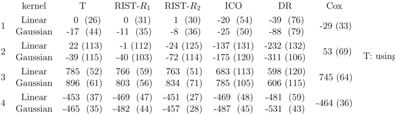
Analysis of non-small-cell lung cancer data: Mean (sd) of value function . . . 63

4.3

Analysis of non-small-cell lung cancer data: Mean (sd) of a clinical measure . . . 64

A.1 Simulation results: Mean and standard deviation of mean log survival time

for different treatment regimes. Censoring rate: 30% . . . 101

LIST OF FIGURES

3.1

Monte Carlo samples of fiducial distributions . . . 30

3.2

Fiducial samples for uncertainty quantification . . . 31

3.3

An example of 95% pointwise and curvewise confidence intervals of survival

function by proposed log-linear interpolation approach. . . 33

3.4

Error rates: survival time follows

Exp

(10)

, and censoring time follows

Exp

(50)

. . . 41

3.5

Error rates: survival time follows

Exp

(10)

, and censoring time follows

Exp

(25)

. . . 42

3.6

Gastric tumor study . . . 44

4.1

Boxplots of mean log survival time for different treatment regimes.

Censor-ing rate: 45% . . . 61

4.2

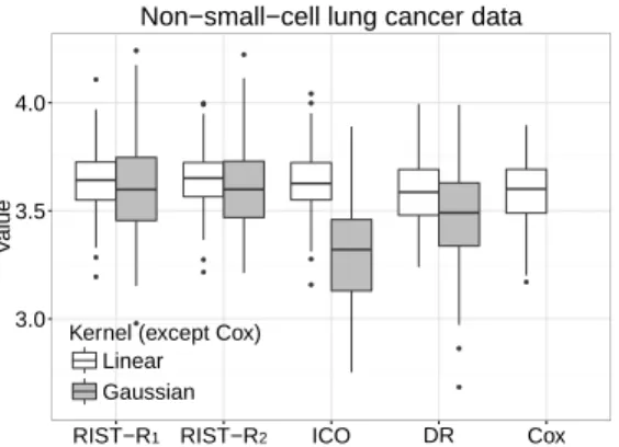
Boxplots of cross-validated value of survival weeks on the log scale . . . 64

4.3

Boxplots of cross-validated restricted mean value of survival weeks on the log scale . . . 65

A.1 Boxplots of mean log survival time for different treatment regimes.

Censor-ing rate: 30% . . . 102

CHAPTER 1

Introduction

In this chapter, we outline the contributions in the subsequent development of the thesis.

1.1

Some asymptotic results for survival tree and forest models

In Chapter 2, we develop a theoretical framework and asymptotic results for survival tree and

forest models under right censoring. We first investigate the method from the aspect of splitting

rules, where the survival curves of the two potential child nodes are calculated and compared. We

show that existing approaches lead to a potentially biased estimation of the within-node survival

and cause non-optimal selection of the splitting rules. This bias is due to the censoring distribution

and the non i.i.d. sample structure within each node. Based on this observation, we develop an

adaptive concentration bound result for both tree and forest versions of the survival tree models.

The result quantifies the variance component for survival forest models. Furthermore, we show with

two specific examples how these concentration bounds, combined with properly designed splitting

rules, yield consistency results. The two examples are: 1) a finite dimensional setting with random

splitting rules; and 2) an infinite dimensional case with marginal signal checking. The development

of these results serves as a general framework for showing the consistency of tree- and forest-based

survival models.

1.2

Nonparametric generalized fiducial inference for survival functions under

censor-ing

survival function under right censoring. We find that the resulting fiducial distribution gives rise to

surprisingly good statistical procedures applicable to both one sample and two sample problems. In

particular, we use the fiducial distribution of a survival function to construct pointwise and curvewise

confidence intervals for the survival function, and propose tests based on the curvewise confidence

interval. We establish a functional Bernstein-von Mises theorem, and perform thorough simulation

studies in various scenarios with different levels of censoring. The proposed fiducial based confidence

intervals maintain coverage in situations where asymptotic methods often have substantial coverage

problems. Furthermore, the average length of the proposed confidence intervals is often shorter

than the length of competing methods that maintain coverage. Finally, the proposed fiducial test

is more powerful than various types of log-rank tests and sup log-rank tests in some scenarios. We

illustrate the proposed fiducial test comparing chemotherapy against chemotherapy combined with

radiotherapy using data from the treatment of locally unresectable gastric cancer.

1.3

Tree based weighted learning for estimating ITRs with censored data

CHAPTER 2

Some asymptotic results for survival tree and forest models

2.1

Introduction

Random forests [19] have become one of the most popular machine learning tools in recent years.

Many extensions of random forests [106, 73, 26, 93] have seen tremendous success in statistical and

biomedical related fields [85, 105, 14, 60, 100, 114, 71] in addition to many applications to artificial

intelligence and machine learning problems.

The main advantage of tree- [21] and forest-based models is their nonparametric nature.

How-ever, the theoretical properties have not been fully understood yet to date, even in the regression

settings, although there has been a surge of research on understanding the statistical properties of

random forests in classification and regression. [83] is one of the early attempts to connect random

forests to nearest neighbor predictors. Later on, a series of work including [12, 11, 54] and [92]

established theoretical results on simplified tree-building processes or specific aspects of the model.

More recently, [142] established consistency results based on an improved splitting rule criteria; [125]

analyzed the confidence intervals induced from a random forest model; [84] established connections

with Bayesian variable selection in the high dimensional setting; [110] showed consistency of the

original random forests model on an additive structure; and [126] studied the variance component of

random forests and established corresponding concentration inequalities. For a more comprehensive

review of related topics, we refer to [13].

in genetic and clinical studies. For a general review of related topics, including single-tree based

survival models , we refer to [16]. To the best of our knowledge, the only consistency result to date is

given in [72] who considered the setting where all predictors are categorical. Hence, in this chapter,

we attempt to lay out a theoretical framework for tree- and forest-based survival models in a general

setting, including when the number of dimensions diverges with the sample size. Furthermore, we

establish consistency under several specific models. Without the risk of ambiguity, we refer to

all considered models as tree-based survival models, while the established results apply to both

single-tree and forest versions.

The chapter is organized as follows: in Section 2.2, we introduce tree-based survival models

and some basic notations. Section 2.3 is devoted to demonstrating a fundamental property of the

survival tree model associated with splitting rule selection and terminal node estimation. A

concen-tration inequality of the Nelson-Aalen [1] estimator based on non-identically distributed samples is

established. Utilizing this result, we derive adaptive concentration bounds for tree-based survival

models in Section 2.4. Furthermore, in Section 2.5, we establish consistency and a variance bound

for two particular choices of splitting rules, one of which are infinite dimensional cases, and one

of which is finite dimensional. Details of proofs are given in the appendices, and a summary of

notation is given before the appendices for convenience.

2.2

Tree-based survival models

The essential ingredient of tree-based survival models is recursive partitioning. A

d-dimensional

feature space

X

is partitioned into terminal nodes, or more precisely, mutually exclusive and

ex-haustive subsets. We denote

A

=

{

A

}

to be the collection of these terminal nodes returned by

fitting a single tree, where

U

is a set of indices, and hence

X

=

S

u∈U

A

and

A

∩

A

=

∅

for any

u

6

=

l. We also call

A

a partition of the feature space

X

. In a traditional tree-building process [21],

where binary splitting rules are used, all terminal node are (hyper)rectangles, i.e.,

A

=

N

j=1

(

a

, b

]

.

identically distributed. Before giving a general algorithm of tree-based survival models, we first

introduce some notation.

Following the standard notation in the survival analysis literature, let

{X

, Y

, δ

}

be a set of

n

i.i.d. copies of the covariates, observed survival time, and censoring indicator, where the observed

survival time

Y

= min(

T

, C

, and

δ

=

1

(

T

≤

C

. We assume that each

T

follows a conditional

distribution

F

t

) =

pr

(

T

≤

t

|

X

, where the survival function is denoted

S

t

) = 1

−

F

t

)

, the

cumulative hazard function

Λ

(

t

) =

−

log

{S

(

t

)

}, and the hazard function

λ

(

t

) = dΛ

(

t

)

/

d

t. The

censoring time

C

’s is assumed to follow the conditional distribution

G

(

t

) =

pr

(

C

≤

t

|

X

)

, where

a non-informative censoring mechanism,

T

⊥

C

|

X

, is assumed.

In any tree-based survival model, terminal node estimation is a crucial part. For any node

A

, this can be obtained through the Kaplan-Meier [74] estimator for the survival function or the

Nelson-Aalen [99, 1] estimator of the cumulative hazard function based on the within-node data.

Our focus in this chapter is on the following Nelson-Aalen estimator

b

Λ

(

t

) =

P

s≤t

P

i=1

1

(

δ

= 1)

1

(

Y

=

s

)

1

(

X

∈

Au)

P

i=1

1

(

Y

≥

s

)

1

(

X

∈

A

)

,

(2.1)

and the associated Nelson-Altshuler estimator [4] for the survival function when needed:

b

S

(

t

) = exp

−

Λ

b

(

t

)

.

Hence a single tree model can be expressed by a collection of doublets

{

A

,

Λ

b

}

.

In

an ensemble survival tree method [73, 141], a set of

B

trees are fitted to the data. In practice,

B

= 1000

is used in the popular

R

package

randomForestSRC

as the default value. Hence the

forest, or a collection of partitions,

{{

A

u

,

Λ

b

}

}

B

b=1

indexed by

b

is constructed. These trees

Algorithm 1:

Pseudo algorithm for tree-based survival models

Input: Training dataset

D

, terminal node size

k, number of trees

B;

Output:

{{

A

,

Λ

b

u

}

}

B b=1

1

for

b

= 1

to

B

do

2

Initiate

A

=

X

, a bootstrap sample

D

of

Dn

,

K

=

∅,

u

= 1

;

3

At a node

A

, if

P

i∈Dbn

1

(

X

∈

A)

< k, proceed to Line 5. Otherwise, construct a

splitting rule such that

A

=

A

∪

A

, where

A

∩

A

=

∅. ;

4

4

Send the two child nodes

A

and

A

to Line 3 separately;

5

Conclude the current node

A

as a terminal node

A

, calculate

Λ

b

u

using the

within-node data, and update

K

=

K

∪ {u}

and

u

=

u

+ 1

;

6

end

7

return

{{

A

,

Λ

b

u

}

}

B b=1

2.3

The splitting rule and its biasedness

One central idea throughout the survival tree and forest literature is to construct certain

goodness-of-fit statistics that evaluate the impurity reduction across many candidate splitting rules.

The best splitting rule is then selected and implemented to partition the node. This essentially

re-sembles the idea in a regression tree setting where the mean differences or equivalently the variance

reduction is used as the criterion. The most popular criteria in survival tree models is

construct-ed through the log-rank statistic [59, 28, 81, 43, 73, 141] and other nonparametric comparisons of

two curves, such as the Kolmogorov-Smirnov, Wilcoxon-Gehan and Tarone-Ware type of statistics

[29, 111]. Other ideas include likelihood or model based approaches [27, 36, 87, 2, 120, 43], inverse

probability of censoring weighting (IPCW) [94, 69], and non-standard criteria such as [134] and

[Krętowska]. [16] provides a comprehensive review of the methodological developments of survival

tree models.

2.3.1

Within-node estimation

To begin our analysis, we start by investigating the Kaplan-Meier (KM) and the

Nelson-Altshuler (NA) estimators of the survival function. There are two main reasons that we revisit

these classical methods: first, these methods are wildly used for terminal node estimation in fitted

survival trees. Hence, the consistency of any survival tree model inevitably relies on their

asymp-totic behavior; second, the most popular splitting rules, such as the log-rank, Wilcoxon-Gehan and

Tarone-Ware statistics, are all essentially comparing the KM curves across the two potential child

nodes, which again plays an important role in the consistency results. We note that although other

splitting criteria exist, our theoretical framework can be extended to address their particular

prop-erties. Without making restrictive distributional assumptions on the underlying model, our results

shows that the currently implemented splitting rules, not surprisingly, are affected by the

under-lying censoring distribution, and are essentially biased, in the sense that they may not select the

most important variable to split on asymptotically. Furthermore, we exactly quantify this biased

estimator by developing a concentration bound around its true mean.

Noticing that the KM and the NA estimators are the two most commonly used estimators, the

following Lemma bounds their difference through an exact inequality regardless of the underlying

data distribution. The proof follows mostly from [34], and is given in the Appendices.

Lemma 1.

Let

S

b

(

t

)

and

S

b

(

t

)

be the Kaplan-Meier and the Nelson-Altshuler estimators,

re-spectively, obtained using the same set of samples

{Y

, δ

}

. Then we have,

|

S

b

(

t

)

−

S

b

(

t

)

|

<

S

b

(

t

)

4

P

i=1

1

(

Y

≥

t

)

,

for any observed failure time point

t

such that

S

b

(

t

)

>

0

.

Assumption 1.

There exists fixed positive constants

τ <

∞

and

M

∈

(0

,

1)

, such that

pr

(

Y

≥

τ

|

X

≥

M,

uniformly for all

X

∈

X

.

Note that similar assumptions are commonly used in the survival analysis literature, for

exam-ples, pr

(

T

≥

τ

)

>

0

in [50], and pr

(

C

=

τ

)

>

0

in [95]. The above assumption is a straightforward

extension due to the partitioning nature of tree models.

2.3.2

A motivating example

Noting that the splitting rule selection process essentially compares the survival curves computed

from two child nodes, we take a closer look at this process. In fact, most studies of the large sample

property of the KM estimator assume that the observations are i.i.d. [22, 56], or at least one set

of the failure times or censoring times are i.i.d. [139]. However, this is almost always not true

for tree-based methods at any internal node because both

T

’s and

C

’s typically depend on the

covariates. The question is whether this affects the selection of the splitting rule. A simulation

study can be utilized to better demonstrate this issue.

Consider the split at a particular node. We generate three random variables:

X

,

X

and

X

from a multivariate normal distribution with mean 0 and variance

Σ

, where the diagonal

elements of

Σ

are all 1, and the only nonzero off diagonal element is

Σ

= Σ

= 0

.

8

. The failure

distribution of

T

is exponential with mean

exp(1

.

25

·

X

+

X

−

2)

. We consider two censoring

distributions for

C: the first one is an exponential distribution with mean 1 for all subjects, i.e.,

they are identically distributed; and the second one is an exponential distribution with mean equal

to

exp(3

·

X

)

. The splitting rule is searched for by maximizing the log-rank test statistics between

the two potential child nodes

{X

_≤

_{c, X}

_∈

_A

_}

_and

_{X

_{> c, X}

_∈

_A

_{}, and the cutting point}

_c

this on the consistency of the entire tree is much more involved since the entire tree structure can

be altered by the censoring distribution. It is difficult to draw a definite conclusion at this point,

but the impact of the censoring distribution is clearly demonstrated.

Table 2.1: Probability of selecting the splitting variable.

Censoring distribution

X

X

X

G

identical

0.950

0.004

0.046

G

depends on

X

0.256

0.028

0.716

2.3.3

Survival estimation based on independent but non-identically distributed

ob-servations

It now seems impossible to analyze the consistency without exactly quantifying the within node

estimation performance. We look at two different quantities corresponding to the two scenarios

used above. The first one is an averaged cumulative hazard function within any node

A

:

Λ

(

t

) =

1

µ

(A)

Z

x∈A

Λ(

t

|

x

)

dP

(

x

)

,

(2.2)

where P is the distribution of

X, and

µ

(A) =

R

x∈A

dP

(

x

)

is the measure of node

A

. Clearly,

since in the first case, the censoring distribution is not covariate dependent, we are asymptotically

comparing

Λ

(

t

)

on the two child nodes, which results in the selection of the first variable. This

should also be considered as a rational choice since

X

contains more signal at the current node.

In the second scenario, i.e., the dependent censoring case, the within-node estimator

Λ

b

(

t

)

does

not converge to the

Λ

(

t

)

in general, which can be inferred from the following theorem. As the

Theorem 1.

Let

Λ(

b

t

)

be the Nelson-Aalen estimator of the cumulative hazard function from a

set of

n

independent samples

{Y

, δ

}

subject to right censoring, where the failure and censoring

distributions (not necessarily identical) are given by

F

’s and

G

’s. Under Assumption 1, we have

for

n

≥

288

/

(

M

)

,

pr

sup

Λ(

b

t

)

−

Λ

∗ n

(

t

)

>

<

16(

n

+ 2) exp

n

−nM

4

288

o

,

(2.3)

where

Λ

(

t

) =

Z

0

P

[1

−

G

(

s

)]

dF

(

s

)

P

[1

−

G

(

s

)][1

−

F

(

s

)]

.

(2.4)

The proof is deferred to Appendix. Based on Theorem 1, if we restrict ourselves to any node

A

, the difference between the within-node estimator

Λ

b

(

t

)

and

Λ

(

t

) =

Z

0

P

Xi∈A

[1

−

G

(

s

)]

dF

s

)

P

Xi∈A

[1

−

G

(

s

)][1

−

F

(

s

)]

(2.5)

is bounded above, where

Λ

(

t

)

is some version of the underlying true cumulative hazard

contami-nated by the censoring distribution. Noting that

Λ

(

t

)

also depends on the sampling points

X

’s,

we further develop Lemma 14 in the Appendix to verify that

Λ

(

t

)

and its expected version

Λ

(

t

)

are close enough, where

Λ

(

t

) =

Z

0

E

[1

−

G

(

s

|

X

)]

dF

(

s

|

X

)

E

[1

−

G

(

s

|

X

)][1

−

F

(

s

|

X

)]

.

(2.6)

It is easy to verify that the difference between

Λ

(

t

)

and

Λ

(

t

)

will vanish if the

F

’s are identical

within a node

A

(a sufficient condition):

Λ

(

t

) =

Z

0

P

Xi∈A

[1

−

G

(

s

)]

P

Xi∈A

[1

−

G

s

)]

dF

(

s

)

1

−

F

(

s

)

(

if

F

≡

F

for all

X

∈

A)

=

Z

0

dF

(

s

)

1

−

F

(

s

)

=

1

µ

(A)

Z

x∈A

Z

0

dF

(

s

)

As we demonstrated in the simulation study above, comparing

Λ

b

(

t

)

between the two child

nodes may lead to a systematically different selection of splitting variables than using

Λ

(

t

)

which

can’t be known a priori. The main cause of the differences between these two quantities is that the

NA estimator treats each node as a homogeneous group, which is typically not true. Another simple

interpretation is that although the conditional independence assumption

T

⊥

C

|

X

is satisfied, we

have instead at each internal node that

T

6⊥

C

|

1

(

X

< c

)

is almost always true for any

j

and

c, causing a nonidentifiability problem.

Exactly quantifying the statistical behavior of each internal node in the entire survival tree

or forest is difficult due to the fact that some subtle changes in the censoring distribution

G

may

completely alter the entire tree structure. Of course, such a difficulty only arises when the splitting

rule is highly data dependent as happens, e.g., with the log-rank test statistic. When the splitting

rule is independent of the observed data, the analysis becomes much easier. We will provide the

results under this random splitting rule setting in Section 2.5. An analog of this result for the

uncensored regression and classification settings was proposed by [20], and further analyzed by

[83, 11, 6] and many others. Another situation where consistency can be derived is when the splitting

rules find almost always the correct variable to split. To look closer at this setting, we consider two

high dimensional cases in Section 2.5, and show that the marginal screening type of splitting rules

will lead to consistency. To establish these results, we use the variance-bias breakdown, and start

by analyzing the variance component of a survival tree estimator in the next section.

2.4

Adaptive concentration bounds of survival trees and forests

In this section, we focus on quantifying the survival tree model from a new angle, namely, the

adaptive concentration [126] of each terminal node estimator to the true within-node expectation.

In the sense of the variance-bias breakdown, this section is to quantify a version of the variance

component of a tree-based model estimator. To be precise, with large probability, our main results

bound

b

Λ

(

t

)

−

Λ

(

t

)

across all potentially possible terminal nodes

A

in a fitted tree or forest. The

adaptiveness comes from the fact that the target of the concentration is the censoring contaminated

version

Λ

(

t

)

, which is adaptively defined for each node

A

with the observed samples, rather than

as a fixed universal value.

The results in this section have many implications.

This bound is essentially the variance

part in a bias-variance break down of an estimator, and is satisfied regardless of the splitting rule

selection. Hence, we can then analyze the bias part to show the consistency of a survival tree

model. Furthermore, following our framework, the consistency results for any survival tree model

can simply be established by checking several conditions on the splitting rules. Although this may

still pose challenges in certain situations, our unified framework is largely applicable to most existing

methods. Some additional definitions and notations are needed as we proceed.

2.4.1

Additional definitions

Following our previous assumptions on the underlying data generating model, we observe a set

of

n

i.i.d. samples

D

=

{X

, Y

, δ

}

. We view each tree as a partition of the feature space,

denoted

A

=

{

A

}

, where the

A

’s are non-overlapping hyper-rectangular terminal nodes. The

following definition of a valid partition, which we owe to [126], is used to restrict the partition

A

being constructed. Here we state the definition again:

Definition 2.1 Valid tree and forest partitions [126].

A tree partition

A

is

{α, k}-valid if it

satisfies two conditions: 1). For each splitting, the child node contains at least a fraction

α

∈

(0

,

0

.

5)

of the training samples in its parent node; and 2). Each terminal node contains at least

k

training

examples. For the training data

D

, we denote the set of all

{α, k}-valid tree partitions by

V

(D)

.

In addition, define the collection

{

A

}

b=1

as a valid forest partition if all of the

B

partitions

A

’s

The following definition is essentially the tree model estimator of the cumulative hazard function

obtained form a partition

A

. When

A

∈

V

(D)

, we will call the induced estimator a

valid survival

tree

. The regression version of their definitions can be found in [126].

Definition 2.2 Valid survival tree.

Given the observed data

D

, a valid survival tree estimator

of the cumulative hazard function is induced by a valid partition

A

∈

V

(D

)

with

A

=

{

A

}

:

b

Λ

(

t

|

x

) =

X

u∈U

1

(

x

∈

A

Λ

b

(

t

)

,

(2.8)

where each

Λ

b

(

t

|

x

)

is defined in Equation (2.1).

When an ensemble of trees are fitted, we define a

valid survival forest

:

Definition 2.3 Valid survival forest.

A valid survival forest

Λ

b

(b)}B1

is defined as the average

of

B

valid survival trees induced by a collection of valid partitions

{

A

}

∈

H

(D

:

b

Λ

(b)}B1

(

t

|

x

) =

1

B

B

X

b=1

b

Λ

(

t

|

x

)

.

(2.9)

In the following, we define the censoring contaminated survival tree and forest, which are the

asymptotic versions of the corresponding within-node average estimators of the cumulative hazard

function. Note that by Theorem 1, these averages are censoring contaminated versions

Λ

(

t

)

, but

not the true averages

Λ

(

t

)

.

Definition 2.4 Censoring contaminated survival tree and forest.

Given the observed data

D

and

A

∈

V

(D

)

, the corresponding censoring contaminated survival tree is defined as

Λ

(

t

|

x

) =

X

1

(

x

∈

Au)Λ

(

t

)

,

(2.10)

where each

Λ

u,n

(

t

)

is defined by Equation (2.5). Furthermore, let

{

A

}

B

1

∈

H

(D

. Then the

censoring contaminated survival forest is given by

Λ

(b)}B1, n

(

t

|

x

) =

1

B

B

X

b=1

Λ

2.4.2

Main result

In order to obtain the adaptive concentration bound for survival trees, we need to bound

b

Λ

(

t

|

x

)

−

Λ

(

t

|

x

)

for all valid partitions

A

∈

V

(D

)

. We first specify several regularity assumptions. The first

assumption is a bound on the dependence of the individual features. Note that in the literature,

uniform distributions are often assumed [12, 11] on the covariates, which implies independence. To

allow dependency among covariates, we assume the following, which has also been considered in

[126].

Assumption 2.

Covariates

X

∈

[0

,

1]

are distributed according to a density

p

(

·

)

satisfying

1

/ζ

≤

p

(

x

)

≤

ζ

for all

x

and some

ζ

≥

1

.

We also set a restriction on the tuning parameter—the minimum terminal node size

k—so that

it grows with

n

and dimension

d

via the following rate:

Assumption 3.

Assume that

k

is bounded below so that

lim

log(

n

) max

{

log(

d

)

,

log log(

n

)

}

k

= 0

.

(2.12)

Then we have the adaptive bound for our tree estimator in the following theorem. The proof is

presented in Appendix.

Theorem 2.

Suppose the training samples

(

X

, Y

, δ

)

satisfy Assumptions 1 and 2, and the rate of

the sequence

(

n, d, k

)

satisfies Assumption 3. Then all valid trees concentrate on censoring

contam-inated tree:

sup

α,k(Dn)

Λ

b

(

t

|

x

)

−

Λ

∗

A,n

(

t

|

x

)

≤

M

s

log(

n/k

)[log(

dk

) + log log(

n

)]

k

log((1

−

α

)

₎

,

In addition, in a high dimensional setting, i.e.

lim inf

n→∞

(

d/n

)

>

0

, Theorem 2 can be simplified as

follows:

Corollary 1.

Suppose the training samples

(

X

, Y

, δ

)

satisfy Assumptions 1 and 2, and the rate of

sequence

(

n, d, k

)

satisfies Assumption 3 and

lim inf

n→∞

(

d/n

)

>

0

. Then all valid trees concentrate on

censoring contaminated trees:

sup

α,k(Dn)

Λ

b

(

t

|

x

)

−

Λ

∗

A,n

(

t

|

x

)

≤

M

s

log(

n

) log(

d

)

k

log((1

−

α

)

₎

,

with probability larger than

1

−

2

/

√

n

, for some universal constant

M

.

Remark 2.4.1.

In a moderately high dimensional setting, i.e.

d

∼

n, the rate is

log(

n

)

/k

. In

an ultra high dimensional setting, for example,

log(

d

)

∼

n

, where

0

< ϑ <

1

, the rate is close to

n

_/k

_{. The rate that}

_k

_{grows with}

_n

_{cannot be too slow in order to achieve the bound in the}

ultra high dimensional setting. This is somewhat intuitive since if

k

grows slowly then we are not

able to bound all possible nodes defined in 2.1.

The above theorem and corollary hold for all single tree partitions in

V

. Consequently,

we have the following results for the forest estimator. The proof is deferred to Appendix.

Corollary 2.

Suppose Assumptions 1-3 hold. Then all valid forests concentrate on the censoring

contaminated forest probability with larger than

1

−

2

/

√

n

,

sup

(b)}B1∈Hα,k(Dn)

Λ

b

(

t

|

x

)

−

Λ

∗

{A(b)}B1, n

(

t

|

x

)

≤

M

s

log(

n/k

)[log(

dk

) + log log(

n

)]

k

log((1

−

α

)

₎

,

for some universal constant

M

. Furthermore, if

lim inf

n→∞

(

d/n

)

→ ∞

,

sup

(b)}B1∈Hα,k(Dn)

Λ

b

(

t

|

x

)

−

Λ

∗

{A(b)}B1, n

(

t

|

x

)

≤

M

s

log(

n

) log(

d

)

with probability larger than

1

−

2

/

√

n

, for some universal constant

M

.

The results established in this section essentially address the variation component in a fitted

random forest. We chose not to use the true within-node population averaged quantity

Λ

(

t

)

(see

Equation 2.6), or its single tree and forest versions as the target of the concentration. This is

because such a result would require bounded density function of the failure time

T

. However, when

f

(

t

)

is bounded, the results can be easily generalized to

Λ

(

t

)

. Lemma 2 provides an analog of

Theorem 1 in this situation.

The next section establishes consistency of several specific models. Intuitively, if a particular

splitting rule leads to “nicely behaved” terminal nodes across the entire tree or forest, then

consis-tency results can be derived. For example, for a finite dimensional case, “nicely behaved” terminal

nodes essentially require that the diameter of each terminal node shrinks to 0 (in the language

of [38]), while in a high-dimensional case, we would require that the diameters of all important

variables (see definition in Section 2.5.2 below) shrink to 0.

2.5

Consistency of survival tree and forest models

2.5.1

Consistency of survival forest when dimension

d

is fixed

In this setting, we assume the dimension of the covariates space is fixed and finite. At each

internal node we choose the splitting variable randomly. When the splitting variable is chosen, we

choose the splitting point at random such that both two child nodes contain at least a proportion

α

of the samples in the parent node. To prove the consistency of the forest, we need to bound the

bias term

sup

E

Λ

∗

{A(b)}B1, n

(

t

|

X

)

−

Λ(

t

|

X

)

,

and combine the results with the variance aspect. It should be noted that in Section 2.4, we did

not treat the tree- and forest- structures (

A

and

{

A

}

) as random variables. Instead, they were

treated as elements of the valid structure sets. However, in this section, once a particular splitting

rule is specified, these structures become random variables associated with certain distributions

induced from the splitting rule. When there is no risk of ambiguity, we inherit the notation

Λ

b

to represent a tree estimator, where the randomness of

A

is understood as part of the randomness

in the estimator itself. A similar strategy is applied to the forest version of the estimator. Before

presenting the consistency results, we introduce an additional smoothness assumption on the hazard

function:

Assumption 4.

For any fixed time point

t

, the cumulative hazard function

Λ(

t

|

x

)

is

L

-Lipschitz

continuous in terms of

x

, and the hazard function

λ

(

t

|

x

)

is

L

-Lipschitz continuous in terms of

x

,

i.e.,

|

Λ(

t

|

x

)

−

Λ(

t

|

x

)

| ≤

L

||x

−

x

||

and

|λ

(

t

|

x

)

−

λ

(

t

|

x

)

| ≤

L

kx

−

x

k

, respectively,

where

k · k

is the Euclidean norm.

We are now ready to state our main consistency results for the proposed survival tree model.

Theorem 3 provides the point-wise consistency result. The proof is presented in Appendix.

Theorem 3.

Under the assumptions 1–4, the proposed survival tree model with random splitting

rule is consistent, i.e., for each

x

,

sup

b

Λ

(

t

|

x

)

−

Λ(

t

|

x

)

=

O

s

log(

n/k

)[log(

dk

) + log log(

n

)]

k

log((1

−

α

)

₎

+

k

n

with probability approaching to 1, where the constants

0

< c

, c

<

1

,

c

= (1

−

2

α

)

/

8

and

c

=

c3(1−c2)(1−c4)

log1−α(α)

. Consequently,

sup

E

|b

Λ

(

t

|

X

)

−

Λ(

t

|

X

)

|

=

O

s

log(

n/k

)[log(

dk

) + log log(

n

)]

k

log((1

−

α

)

₎

+

k

n

+ log(

k

)

w

,

where

w

=

2

√

n

+

d

exp

n

−

c

2

2

log

(

n/k

)

2

d

o

+

d

exp

n

−

(1

−

c

)

c

c

2

4

log

(

n/k

)

2

d

o

.

Remark 2.5.1.

The first part

q

log(n/k)[log(dk)+log log(n)]

klog((1−α)−1₎

comes from the concentration bound results

and the second part

(

)

comes from the bias part. We point out that the optimal rate is obtained

by setting

k

=

n

c₃

c₃₊₁/2d_log1−α(α)

_{, and then the optimal rate is close to}

_n

c₃

2[c₃₊₁/2d_log1−α(α)]

_{. If we}

always split at the middle point at each internal node, then the optimal rate degenerates to

n

_,

which is the same rate as in [32].

The consistency result can be easily extended to survival forests with

B

trees. Theorem 4

presents an integrated version, which can be derived from Theorem 3.

Theorem 4.

Under the Assumptions 1-4, the proposed survival forest is consistent, i.e.

lim

B→∞

sup

E

|b

Λ

(

t

|

X

)

−

Λ(

t

|

X

)

|

=

O

s

log(

n/k

)[log(

dk

) + log log(

n

)]

k

log((1

−

α

)

₎

+

k

n

+ log(

k

)

w

,

where

w

is a sequence approaching to 0 as defined in Theorem 3,

0

< c

, c

<

1

,

c

= (1

−

2

α

)

/

8

and

c

=

1−α(α)

.

2.5.2

Consistency of survival forests with a nonparametric splitting rule when

dimen-sion

d

is infinite

model has size

|M|

=

d

≤

d. We implement the splitting rule as following. A similar idea for

splitting rules has been considered in the guess-and-check forest [126] in the regression setting.

Algorithm 2:

Splitting rule for marginal checked survival forest

1

1

For a currently internal node

A

containing at least

2

k

training samples, we pick a splitting

variable

j

∈ {

1

, . . . , d}

uniformly at random;

2

2

We then pick the splitting point

x

˜

using the following rule such that both two child nodes

contain at least proportion

α

of the samples in their parent node:

˜

x

= arg max

∆(

x

)

,

where

∆(

x

) =

R

b

Λ

j(x)

(

t

)

−

b

Λ

j(x)

(

t

)

dt,

A

j

(

x

) =

{X

:

X

≥

x}, and

A

(

x

) =

{X

:

X

< x},

X

is the

j-th dimension of

X;

3

3

If either there is already a successful split on the variable

j

or the following inequality holds:

∆(˜

x

)

≥

2

M

τ

s

log(

n/k

)[log(

dk

) + log log(

n

)]

k

log((1

−

α

)

₎

,

for a universal constant

M

then we split at

x

˜

along the

j-th variable. If not, we randomly

sample another variable out of the remaining variables and proceed to Step 2). When there

are no remaining feasible variables, we randomly select an index out of

d

to proceed to a split.

Lemma 3 and 4 show that a

d

dimensional survival forest based on the above splitting rule

is equivalent to a

d

dimensional survival forest with probability approaching to 1.

Λ

(

t

)

is an

essential tool to prove Lemma 3 and 4. Notice that

Λ

(

t

)

is a sample version of the asymptotic

distribution of the terminal node

A

. In Lemma 2, we show the bound of the difference of

Λ

(

t

)

and its integrated version

Λ

(

t

)

across all valid nodes

A

, where

Λ

(

t

)

is as defined in Equation 2.6.

The proof is given in Appendix.

Lemma 2.

Assume the density function of the failure time

f

(

t

|

x

)

is bounded by

L

for each

x

.

The difference between

Λ

(

t

)

and

Λ

(

t

)

is bounded by

sup

α,k(Dn)

Λ

(

t

|

x

)

−

Λ

(

t

|

x

)

≤

M

s

log(

n/k

)[log(

dk

) + log log(

n

)]

k

log((1

−

α

)

₎

,

with probability larger than

1

−

1

/

√

n

.

Lemma 3.

The probability that the proposed survival tree ever splits on a noise variable is smaller

than

3

/

√

n

.

To establish consistency, we need one additional assumption about monotonicity of the failure

distribution and the effect size of the censoring distribution.

Assumption 5.

Monotonicity of

dF

. Without loss of generality, assume that

f

=

dF

is monotone

increasing with respect to

X

. Furthermore, there is a minimum effect size

` >

0

such that

Z

0

˜

M

Z

0

R

1/2

f

(

s

|

X

(j)

₌

_x

_{, X}

₌

_x

₎

_dx

R

1/2

[1

−

F

(

s

|

X

=

x

, X

=

x

)]

dx

ds

−

1

˜

M

Z

0

R

0

f

(

s

|

X

=

x

, X

−j)

₌

_x

₎

_dx

R

0

[1

−

F

(

s

|

X

=

x

, X

=

x

)]

dx

ds

dt

≥

`,

for all

x

∈

[0

,

1]

and all important (non-noise) variables

j

. Here,

X

is a sub-vector of

X

obtained by removing the

j

th entry, and

M

˜

stands for the lower probability bound of censoring at

τ

,

i.e.,

pr

(

C

≥

τ

|

X

)

≥

M >

˜

0

.

Recall in Assumption 1, we assumed that pr

(

Y

≥

τ

|X

)

≥

M >

0

. Hence taking

M

˜

as

M

automatically satisfies the above assumption of the censoring distribution; however,

M

˜

is usually

larger than

M. Note that Assumption 5 essentially bounds below the signal size regardless of any

dependency structures between

C

and

T

for a given subject

i. However, when the

G

’s in Equation

2.5 are identical, the constant

M

˜

can be removed from the assumption.

Lemma 4.

At any given internal node, if an important variable is randomly selected and has never

been used before, then the probability that the proposed survival tree splits on this variable is at least

1

−

3

/

√

n

.

Based on Lemma 3 and 4, we essentially only split on

d

dimensions with probability

1

−

3

/

Theorem 5.

Under the Assumptions 1-5, the proposed survival forest using the splitting rule

spec-ified in Algorithm 2 is consistent, i.e.

lim

B→∞

sup

E

|b

Λ

(

t

|

X

)

−

Λ(

t

|

X

)

|

=

O

s

log(

n/k

)[log(

dk

) + log log(

n

)]

k

log((1

−

α

)

₎

+

k

n

+ log(

k

)

w

,

where

w

is a sequence approaching to 0 as defined in Theorem 3,

0

< c

, c

<

1

,

c

= (1

−

2

α

)

/

8

and

c

=

1−α(α)

.

Although we have developed a result where

d

can grow exponentially fast with

n

in this section,

the splitting rule implemented was not a completely the same as the practically used version because

it essentially checks only the signal where the candidate variable have never been used. This is done

by comparing the signal for the two potential splits

X

<

1

/

2

versus

X

<

1

/

2

at an internal

node. Once a variable is first used, it will be automatically included as a candidate thereafter. This

idea is essentially the same as the protected variable set used in [142], where the protected set serves

as the collection of variables that have used in previous nodes.

2.6

Discussion

In this chapter, we developed several fundamental results for tree- and forest-based survival

models. Firstly, we investigated the within-node Nelson-Aalen estimator of the cumulative hazard

function and developed a concentration inequality for independent but non-identically distributed

samples. Secondly, we extended the result to develop a concentration bound across all possible

fitted tree and forest models. Lastly, we developed consistency under two specific models with

corresponding splitting rule methods.

In section 2.5, our results suggest that survival tree models are able to adapt to the sparsity

structure of the underlying model. This is demonstrated in the second consistency results, where

the number of true important variables

d

is much smaller than the total number

d

≥

d

. The