The effect of obesity on labor market outcomes

(1)

THE EFFECT OF OBESITY ON LABOR MARKET OUTCOMES

Euna Han

A dissertation submitted to the faculty of the University of North Carolina at Chapel Hill in partial fulfillment of the requirements for the degree of Doctor of Philosophy in the

Department of Health Policy and Administration.

Chapel Hill 2006

Approved by:

Edward C. Norton, Ph.D. (Advisor) Barry M. Popkin, Ph.D.

Kristin L. Reiter, Ph.D. Sally C. Stearns, Ph.D.

(2)

© 2006

Euna Han

(3)

ABSTRACT

Euna Han: Effect of Obesity on Labor Market Outcomes

(Under the direction of Edward C. Norton)

(4)

(5)

LIST OF TABLES

Table 4.1 Sample sizes, retention rates, and response rates in the NLSY79 ... 49

Table 4.2a Summary statistics for the final sample: women ... 50

Table 4.2b Summary statistics for the final sample: men... 52

Table 4.3 Description of dependent variables ... 54

Table 4.4 Variation in employment status over time by gender and age groups... 55

Table 4.5 Distribution of industry categories according to the Census 1980 codes in the final sample ... 56

Table 4.6 Variation in status of occupations where social interactions with colleagues or customers over time by gender and age groups ... 57

Table 4.7 Within-person variation in four BMI categories in the total and employed sample by gender ... 58

Table 4.8a Within-person variation in four BMI categories in the total sample by age groups... 59

Table 4.8b Within-person variation in four BMI categories in the employed sample by age groups ... 60

Table 4.9 Variations in BMI within and between persons by gender ... 61

Table 4.10 Education level by BMI groups for both genders... 62

Table 5.1 Strength of instruments... 80

Table 5.2 Results from first-stage equations... 81

Table 5.3 Specification tests for instruments... 82

Table 5.4 Specification tests for the instruments for the Arellano-Bond (AB) model ... 83

Table 6.1 Effect of BMI on the probability of employment using the linear probability model ... 95

Table 6.2 Effect of BMI on the probability of employment by age group ... 96

(8)

Table 6.4 Effect of BMI on the probability of having occupations where social

interaction is required by age group ... 98

Table 6.5 Effect of BMI on the hourly wage ... 99

Table 6.6 Effect of BMI on the hourly wage by age group ... 100

Table 6.7a Effect of BMI on the hourly wage by occupation group: men ... 101

Table 6.7b Effect of BMI on the hourly wage by occupation group: women ... 102

Table 7.1a Summary of results by age group: 2SRI with the individual fixed-effects model for the combined sample: Men ... 114

Table 7.1b Summary of results by age group: 2SRI with the individual fixed-effects model for the combined sample: Women... 115

Table 7.2 Summary of results by age group: 2SRI with the individual fixed-effects model for the combined sample: Women... 116

(9)

LIST OF FIGURES

Figure1.1 Trends in Body Mass Index and percentage obese for persons 18 years of age and older in the Behavioral Risk Factor Surveillance System,

1984-1999 ... 10

Figure 4.1 Distribution of BMI over age by gender ... 63

Figure 4.2 Distribution of BMI by BMI categories over age by gender ... 64

(10)

CHAPTER I: INTRODUCTION

Overview

The objective of this study is to understand the effect of obesity on labor market outcomes. The prevalence rate of obesity has increased by over 50% since the late 1970s. Chou, Grossman and Saffer (2002) showed a sharp upward trend in obesity between 1978 and 1991 using nationally representative data. During this thirteen-year period, the number of obese Americans grew by 55%. The previous literature has consistently reported health problems and a high health-related social cost caused by obesity (Sturm, 2002).

Obesity is important for labor market outcomes. Obese people may be discriminated against by consumers or employers due to their distaste for obese people in a job where slimness does not matter. Employers also may not want to hire obese people due to the expected health cost if the employers provide health insurance to their employees (Hamermesh and Biddle, 1994). These employer-side distastes may result in poor labor market outcomes in terms of wage earnings and the low likelihood of being employed, as well as sorting of obese people into jobs where slimness is not rewarded.

(11)

choice. An example of such externality cost is an increase in the insurance premium due to large health services use by obese people (Bhattacharya and Sood, 2005). Individuals do not always make rational choices concerning body weight and the information they can use are not perfect, which provide a rationale for the public intervention (Cawley, 2004). Among several potential policy measures to help individuals’ rational decision regarding the body weight control, disseminating information about the adverse effect of obesity will provide an incentive for an individual to change their behavioral choices relevant to healthy body weight.

This study addresses the following specific research questions: Ceteris paribus, does an increase in BMI: (1) decrease the likelihood of being employed; (2) decrease the likelihood of sorting into occupations where social interaction with customers or colleagues is required; (3) decrease wage earnings; (4) affect wage earnings differently at various stages of the life cycle; and (5) affect wage earnings differently in occupations where social interaction with customers or colleagues is required versus other occupations. These research questions are explored separately by gender.

This study uses the National Longitudinal Survey of Youth (NLSY79), which is suitable to address the relationship between obesity and labor market outcomes with sophisticated statistical techniques. The NLSY79 has detailed information on the labor market outcomes, height, and weight in a panel structure.

(12)

Obesity, which is the key explanatory variable of interest in the study, is endogenous. Individual fixed-effects control for the unobservable individual heterogeneity (like endowment). The endogeneity of obesity is controlled for in two-stage instrument variable estimation models with over-identifying instruments. The identifying instruments for obesity are three state-level variables (fast food prices, beer prices, and sales in restaurants), and two individual-level variables (siblings’ BMI and a five-year lag of the respondents’ BMI).

Trends and causes on obesity

This section contains two sub-sections. First, the growing epidemic of obesity is discussed to emphasize the importance of obesity for public policy. In the second subsection, the endogenous characteristics of obesity are discussed. Individuals make their behavioral choices that may affect their body weight, in particular, diet and exercise. The potential correlation of obesity with labor market outcomes is also discussed in the second sub-section because the correlation also makes obesity an endogenous explanatory variable.

The obesity epidemic

(13)

study by Sturm (2002), social costs of obesity are reported to exceed those of cigarette smoking and alcoholism. Therefore, obesity also affects major public transfer programs such as Medicaid, Medicare, and Social Security (Lakdawalla and Philipson, 2002).

Although weight has been rising in the U.S. throughout the twentieth century, the rise in obesity since the 1980s is fundamentally different from past changes. That is, since the 1980s, weight has grown more than physicians recommend for healthy weight (Cutler, Glaeser, and Shapiro, 2003).

Figure 1.1 depicts annual trends in average Body Mass Index (BMI) (left vertical axis) and in the percentage (right vertical axis) who are obese for persons 18 years and older in the Behavioral Risk Factor Surveillance System during the period between 1984 and 1999. BMI is a measure of height-adjusted weight equal to weight in kilograms divided by squared height in meters. Persons with a BMI equal to or greater than 30 are classified as obese. A BMI between 25 and 30 is classified as overweight, and a BMI below 18.5 is underweight (National Heart, Lung, and Blood Institute, 1998). Annual trends show that the average BMI increased from 1984 to 1998 by 9%, and the number of obese adults more than doubled during the same period (Chou, Grossman, and Saffer, 2002).

(14)

The endogeneity of obesity

Obesity is endogenous because individual choices partly affect the state of being obese besides endowed genetic factors. That is, obesity primarily is a choice variable, not a given variable. In technical terms, obesity as a regressor is not orthogonal to the unobserved characteristics in the error terms in models of labor market outcomes because unobserved individual heterogeneity will affect both labor market outcomes and obesity. Time preference is an example of unobserved individual heterogeneity. Individuals with a high discount rate for future will be less likely to invest in their own human capital such as education, which would be correlated with their own wage earnings. Those individuals with a high discount rate also are less likely to restrain from risky health behaviors including the consumption of fattening food. The discount rate affects both obesity and labor market outcomes. Thus, obesity is an endogenous explanatory variable in the econometric sense.

Several factors have been discussed as contributors to obesity as a choice variable in the previous literature. First, low income or poverty has been claimed to cause being overweight or obese particularly in women (Stunkard, 1996; Sobal and Stunkard 1989). The different distribution of obesity by income level may complicate policy measures for resolving any discrimination against obese people in the labor market (Averett and Koreman, 1996). It has been reported that fast food and convenience food are inexpensive and are high in calories compared to other healthier foods. If more fattening foods are generally cheaper than healthier, non-fattening food, the people with lower income will be more likely to consume fattening foods (Chou, Grossman, and Saffer, 2002).

(15)

inexpensive but fattening convenience and fast food. The real average hourly earnings in the private sector decreased from 1982 to 1995, and it was only 4.5% higher in 2002 than in 1982 (Chou, Grossman, and Saffer, 2002; U.S. Census Bureau, 2003; Bureau of Labor Statistics, 2005). However, previous studies have found that higher household income did not result in better weight outcomes (Chou, Grossman, and Saffer, 2002; Lakdawalla and Philipson, 2002). That result might imply that an increase in participation into the labor force or an increase in work hours for women contributes to weight gain through a decrease in leisure time. In fact, participation rate in the labor force for women increased 12.5% between 1982 and 2002 (Bureau of Labor Statistics, 2005). Those increasing trends of market work will reduce the time and energy available for home production including food preparation, which can also contribute in part to the increasing prevalence of convenience or fast food. Several studies have supported the effect of reduced leisure time for household production on weight gain. For example, a child is more likely to be overweight if her mother worked more hours per week over the child’s life, and that adverse effect of work hours on child’s excess weight is larger for those mothers in high socioeconomic status (Ruhm, 2004; Anderson, Butcher, and Levine, 2003).

(16)

of the extent of obesity, while prices at fast-food restaurants, full-service restaurants had negative and significant effects on the extent of obesity (Chou, Grossman, and Saffer, 2004).

If the fast food market is competitive, then an increase in the number of fast food restaurants will decrease the average price of fast food. The previous literature has displayed systematic dispersion in the number of restaurants or grocery stores in a market by socioeconomics profiles of the market. For example, Stewart and Davis (2005) found that low population and low levels of income might be associated with limited access to restaurants, and thus, higher prices. If the demand for groceries or number of restaurants increases in a market, firms would supply more by opening new stores in the market, ceteris paribus. Kaufman and colleagues (2005) reported higher grocery prices in urban stores than in suburban markets. Spatial concentration of people with a common socioeconomic profile may complicate the dynamic relationship among obesity, socioeconomic status, and food prices. Individuals tend to choose to live near others like themselves, and thus, those with the best opportunities at economic success will cluster together. For example, a high proportion of low income, racial or ethnic minorities tend to live in urban centers, while people with high income tend to live in suburban areas (Toussaint-Comeau and Sherrie, 2002). This possible neighborhood selection in an area by socioeconomic profile implies people with low income may pay higher food prices due to their residential area characteristics, and therefore, more tend to demand cheap substitutes for expensive foods.

(17)

for preparing food. Furthermore, it reduces the time delay before actual consumption of food, which will particularly affect food consumption by people with self-control problems. For those people, a decrease in the delay of instant gratification from food consumption will make it more difficult to pass up current pleasure for future benefits (Cutler, Glaeser, and Shapiro, 2003).

Trends in energy intake have also changed since the 1970s. For example, energy intake from sweetened beverage consumption increased by 135%, while energy intake from milk consumption fell by 38% from 1977 to 2001 for samples aged 2 to 60 years. This corresponds to a 278 total calorie increase during the same period (Nielsen and Popkin, 2004; Popkin, 1996). Other than the source of energy intake, the portions of food have increased as well. Between 1977 and 1996, food portion sizes increased both inside and outside the home for specific food items including salty snacks (from 1.0 to 1.6 oz), soft drinks (13.1 to 19.9 fl oz), french fries (3.1 to 3.6 oz), hamburgers (5.7 to 7.0 oz), and Mexican food (6.3 to 8.0 oz) (Nielsen and Popkin, 2003).

(18)

BMI. Workers in a job requiring physical strength may have strong muscle mass, and thus, greater BMI.

(19)

Figure 1.1 Trends in Body Mass Index and percentage obese for persons 18 years of age and older in the Behavioral Risk Factor Surveillance System, 1984-1999

Source: Chou, Grossman, and Saffer (2002)

Average BMI

(20)

CHAPTER II: LITERATURE REVIEW

The first section of this chapter reviews the previous literature about the effect of obesity on labor market outcomes. Because education is a strong predictor of labor market outcomes, the second subsection discusses the effect of obesity on school-related outcomes. The previous literature studying the effect of physical appearance on labor market outcomes is reviewed in the third subsection, because obesity is one component of looks. In the last section, the significance of the current study including policy implications and how the current study can improve the previous literature is discussed.

How does obesity affect labor market outcomes?

Several studies have linked obesity to labor market outcomes, mostly wages. Even though all of those studies essentially used the same data, the NLSY79, their results differ markedly. These inconsistent trends in the previous literature may be attributed to the lack of valid control for the endogeneity of obesity (Register and Williams, 1992; Loh, 1993; Pagan and Davila, 1997; Gortmaker et al., 1993; Sargent and Blanchflower, 1994).

(21)

suffer obesity penalties in the labor market in terms of low earnings, with a lesser extent for women than for men, even after self-esteem was controlled for. However, their way to control for endogeneity of obesity is not likely to produce valid parameter estimates for the effect of obesity on the labor market outcomes. Their estimation was based on the assumption of no serial inter-temporal correlation in the wage residuals, which is not likely. Although the sister fixed effects sweep out the unobserved permanent endowment factors at the family level belonging to the error term, individually heterogeneous endowment factors will remain unobserved in the error term.

Similar to Averett and Korenman’s (1996) study, Conley and Glauber (2005) took the lag of 13 and 15 years of BMI as instruments for the current BMI, and used the sibling fixed-effects model to control for the endogeneity of BMI. Using the Panel Study of Income Dynamics (PSID) 1986, 1999, and 2001 data, they estimated the effect of obesity on three labor market outcomes: occupational prestige, labor earnings, and total family income. Their study results were consistent with Averett and Korenman (1996) in that obesity penalizes women in terms of not only their own earnings, family income, and occupational prestige, but also spouse’s earnings, and spouse’s occupational prestige. Their study is the only study that measured the effect of obesity on occupational prestige. They measured occupational prestige using Duncan’s Socioeconomics Index (SEI) for 1970 U.S. census occupational classification codes. However, like Averett and Korenman’s (1996) study, they took the lagged BMI as an instrument for obesity with sibling fixed effects. Thus, the limitations of Averett and Korenman’s (1996) study also apply to Conley and Glauber’s (2005) study.

(22)

from the Minnesota Twins Registry. In this study, the identical twin fixed-effects model was used, which eliminated the permanent but unobserved genetic endowments including earnings endowment from the error term. The unobserved earnings endowment in the error term would lead to biased estimators for the effect of BMI on wage, because earning endowment might be correlated with education and a genetic component of body weight. However, if the physical characteristics including BMI were also affected by contemporaneous wage shocks in the error term, then within-twin estimates would still be biased. Therefore, the authors used lagged consumption or the lagged physical characteristics as an instrument for current BMI and height after they swept out time-consistent endowment factors with twin fixed effects.

(23)

on the 2SLS was .00197, and the corresponding absolute value of robust t statistics was 0.19).

Cawley (2000) estimated the effect of obesity on women’s employment disability, which was measured by limitations on the amount of paid work and limitations on types of paid work using 12 years of data from the NLSY79. When the sample women’s own child’s body weight was used as an instrument for the sample women’s body weight, obesity did not have a statistically significant effect on a limitation on the amount of paid work nor a limitation on the type of paid work. Assuming that the instrument in this study is valid, the results imply that loss of body weight among obese women might not reduce the employment disability. However, the validity of the instrument remains untested. Children’s body weight will not be a valid instrument for mother’s body weight if there is unobserved heterogeneity for mothers in the wage residual, which affects both children’s body weight and the mother’s employment disability. For example, smoking or alcohol consumption during pregnancy may reflect the pregnant women’s inconsistent discount rate for the future, which will affect both their performance in their job and their children’s health at birth.

(24)

All of the previous studies focused on the total effect of obesity on wages without identifying indirect pathways linking obesity to different performance in the labor market. A study by Baum and Ford (2004) was one of the two studies trying to estimate the indirect effect of obesity on labor market outcomes.

In a study using 12 years of the NLSY79, they tested four potential pathways linking obesity to labor market outcomes: less productivity due to health problems from obesity, less investment on human capital by obese workers, employers’ distaste for obese employees due to high health care cost for obese people, and consumers’ distaste for obese workers. Their empirical evidence suggested that those pathways might mediate the effect obesity on labor market outcomes. However, the authors did not control for the endogeneity of obesity other than using the individual and family fixed-effects model. If any explanatory variables are not strictly exogenous, i.e., uncorrelated with current and earlier disturbance terms or shocks, then the fixed-effects estimators are inconsistent. Also, they estimated only the intensive marginal effects of those factors in the labor market outcomes in terms of wage, but did not consider the extensive marginal effect, i.e., the effect on labor market participation.

(25)

insurance) was included in the model. The authors argue that this indicates obese workers had lower wages compared to non-obese individuals because of their higher medical expenditure and not because of possible discrimination against obese individuals in the labor market. Their study is a welcome exception for pointing out one potential pathway under the negative effect of obesity on labor market outcomes.

(26)

in terms of low wages. Individual heterogeneity time preference is an example of such factors. Therefore, endogeneity of obesity and employer-provided health insurance should be accounted for in the model. Otherwise, the estimation results would be biased.

How does obesity affect schooling-related outcomes?

One potential pathway for a causal effect of obesity on differentials in the labor market would be differentials in the level of human capital. The previous literature has consistently reported the significant effect of human capital, in particular education or schooling, over the other factors on the outcomes in labor market, although the validity of the estimated causal effect has not been agreed upon (for example, Card, 1994; Angrist and Krueger, 1991). Thus, identifying the effect of obesity on the development of human capital, particularly, schooling-related outcomes, will be highly relevant for policy measures to intervene in any social or economic adverse effect of obesity.

(27)

women, samples in the lighter group have more years of education and higher test scores on average than samples in the heavier group regardless of race.

Likewise, Sargent and Blanchflower (1994) found that obese girls at age 16 had poor performances in math and reading tests in later years than non-obese girls in their study using a British birth cohort. However, they did not find this differential in test scores between the obese and non-obese boys of the same age. This gender differential was also reported in the study by Gortmaker and colleagues (1993) using one year (1981) of the NLSY79. They found that the overweight women in their sample had less education than the non-overweight women, although a differential was not found in the sample of men.

How does beauty affect the labor market outcomes?

Considering that slimness is a component making an individual physically attractive, studies of premiums to overall beauty or stature in the labor market would help to identify any potential consumers’ or employers’ distaste for physically unattractive workers, including obese ones. However, obesity can be a good proxy for beauty in a study for estimating the effect of beauty on labor market outcomes. There is a potential error in the measurement of beauty because standards for beauty are various and rather subjective, while the measurement of obesity is more objective than beauty.

(28)

plainness is larger than the premium of earnings for beauty, and the effects for men are as large as for women. The effect of looks on earnings was found to be independent of the type of occupation. This result might imply no discrimination against plain-looking workers by consumers because consumer-based discrimination may lead to job sorting in the way obese workers choose a job with less interaction with consumers.

For marriage market outcomes, women’s looks were not related to the likelihood of marriage. However, below-average-looking women were more likely to marry men with lower education level than their own attainment. If educational level has a positive effect on earnings in the labor market, this would imply that below-average-looking women face additional economic penalty for bad looks in the form of marrying a husband with potentially lower earnings.

Harper (2000) replicated the study by Hamermesh and Biddle (1994) using U.K. data, and found similar results. It is possible that people with higher earnings are more able to and willing to invest in beauty, and thus, beauty may be endogenous. However, the potential endogeneity problem of looks might be less crucial than obesity because an individual’s looks hardly change during adulthood by any natural way.

(29)

characteristics. The identification for perceived beauty was raised from the respondents’ human capital, and occupational achievement. They found that additional spending on clothing and cosmetics has a positive marginal effect on a woman’s perceived beauty. Moreover, such spending on beauty items was estimated to result in higher earnings for women. However, the sources of identification remained untested.

The effects of beauty on differentials in earnings and career choices were also found in a study by Biddle and Hamermesh (1998) with a longitudinal data on a large homogeneous sample of graduates from one law school. The beauty of each participant of the survey was rated using a book of photographs of matriculants in each entering class. In this study, they found that better-looking attorneys who graduated in the 1970s earned more than others after 5 years of practice. Attorneys in the private sector were better-looking than those in the public sector, and the monetary reward to beauty rose, in particular in the private sector. More attractive men obtained partnership early, and those who moved from public to private sector were more attractive ones while a switch from private to public sector was observed for less attractive ones. Both of the earnings differentials generated by beauty and sorting into the private sector grew as the respondents matured in their practices.

(30)

public-policy intervention is required, and if so, how to implement it to alter any detrimental effect of beauty or other physical characteristics on labor market outcomes (Biddle and Hamermesh, 1998).

Significance of this study

Accurate estimation of the effect of obesity on labor market outcomes will support the understanding of the economic cost of obesity to an individual besides its adverse effect on health. Individuals’ behavioral choices regarding body weight can impose costs not only to the individuals themselves, but also to the others that are not relevant to the choices. An example is the high health care costs for the obese individuals. The rising health expenditure for obese people tolls the other individuals in the same insurance pool via rising insurance premium. If the obese people are under a public insurance, their large consumption of health care resources cost the general public (Bhattacharya and Sood, 2005). Government regulation, such as a special tax for junk food may be needed (or able to) curb the obesity epidemic. However, given that individuals are the ultimate decision-makers for their body weight, raising awareness of the obesity costs to individuals may also be important to reduce the obesity epidemic. Individuals are known to change their behavioral choices more efficiently by a response to the incentives rather than their strong willingness or preferences for changes (French, Story, and Jeffery, 2001; Cawley, 2004). The spillover effect of obesity on labor market outcomes may be able to provide an additional incentive to the individuals to adjust their behavioral choices toward a healthier body weight.

This study will also improve the literature in the following ways:

(31)

conducting the tests of the exogeneity of over-identifying instruments for obesity in the labor market outcome equations besides the tests of the quality of instruments. Thus, this study generates valid parameter estimates of the effect of obesity on labor market outcomes with supported instruments. The individual fixed-effects model is used in conjunction with the two-stage instrument variables estimation model to sweep out any unobserved permanent individual heterogeneity in the error term. Altogether, this study accounts for the feedback effect of labor market outcomes on wages. Within-variation estimators alone would be inconsistent if strict exogeneity fails by feedback effect, that is, if the current obesity level is affected by the prior error term in the equations on labor market outcomes.

2) This study distinguishes the effect of obesity on labor market outcomes at the extensive margin (i.e., employment and occupation choice), as well as at the intensive margin (i.e., wages for participating workers). Although one previous study investigated the effect of obesity on the probability of employment at a so-called white-collar job (Cawley, 2000), the parameter estimates in that study remained untested due to limited controls for the endogeneity of obesity, as discussed earlier. None of the previous literature has estimated the effect of obesity on the occupation choices where obesity may affect the job performances. Furthermore, this study investigates different marginal effect of obesity on hourly wages between occupations where obesity may penalize and other occupations.

(32)

(33)

CHAPTER III: CONCEPTUAL FRAMEWORK

In this chapter, potential underlying factors linking obesity and labor market outcomes are discussed, using related economic theories. Four potential underlying factors for the total effect of obesity on labor market outcomes have been identified: health problems caused by obesity; myopia of obese individuals; consumer-based discrimination against obese workers in the labor market; and employer-based distaste for obese workers with regard to high health care cost for obese people or other factors associated with weight and job productivity. It should be noted, however, that this study focuses on the total effect of obesity on labor market outcomes, rather than estimating the direct effect of obesity on labor market outcomes through the suggested factors. How the potential instruments for obesity would work to identify its effect on labor market outcomes is discussed. Testable hypotheses suggested by the conceptual framework follow.

How does obesity affect labor market outcomes

Health problems for obese people

(34)

people may have worse labor market outcomes than non-obese people, ceteris paribus, because their health problems caused by obesity limit the amount of work or types of work via higher absenteeism or sick leave.

However, the effect of health problems regardless of its causes is not the main interest of this study. An individual’s health status is also endogenous because some health problems can cause obesity itself. Thus, this study excludes person-year observations for any respondent who answered that their health problems limit types of work or amount of work to exclude health problems as a potential mediating factor.

Myopia

Typically, it is assumed that an individual’s time preference is persistent, and thus, her discount rate should be the same over time. However, individuals may discount the near future less heavily than the long-term future when they make decisions over time intervals. That is, those individuals discount future hyperbolically or quasi-hyperbolically (Becker and Murphy, 1988).

(35)

inconsistent time-preference, they become “spendthrift” or myopic with inconsistent or imprudent planning (Strotz, 1955). Thus, myopic people discount the future at a higher rate than the pure time discount rate, while they trade off consumption in future states at the time discount rate (Cutler, Glaeser, and Shapiro, 2003).

If individuals are myopic, they ignore future effects when they make decisions about current consumption (Becker, Grossman, and Murphy, 1994). Food consumption brings immediate gratification, while costs of over-consumption of food occur in the future (Cutler, Glaeser, and Shapiro, 2003). Therefore, myopic workers are less likely to be concerned about long-term adverse health effects of consuming fattening foods at present than non-myopic workers, and accordingly, more likely to be obese (Cawley, 2000).

If the high discounting of future consequences of food consumption is also found in consumption of other goods associated with their human capital, those people will ignore future return to the investments on their human capital, such as on-the-job training, when they make decisions about current consumption of those investments. People with high future discount rates are also likely to participate in risky health behaviors, including smoking and heavy drinking, for the same reason they consume fattening foods. Those potentially less human capital and/or risky behaviors may cause poor labor market outcomes.

Discrimination in the labor market against obese people

(36)

behaviors, including smoking or alcoholism. Consumption of unhealthy fattening foods (or failure to get sufficient exercise) is a risky health behavior that is more likely to be observable than consumption of other risky health behaviors. That is, consumption of fattening unhealthy foods mostly yields obesity, which is quite visible. An unhealthy risk behavior may be correlated with any other unhealthy behaviors if individuals with high discount rate are more likely to consume those behaviors. Therefore, any existing discrimination against obese people may come from only discrimination against consumption of fattening unhealthy foods (or failure to get sufficient exercise), overall discrimination against any type of risky health behaviors, or a high discount rate. Also, discrimination against obese people can result from consumer-based distastes for obese workers, or employer-based distaste regardless of their overall preference for people performing risky health behaviors. Regardless of the underlying reasons for discrimination against obese people, the discrimination in the labor market would result in poorer labor market outcomes for obese people than non-obese people.

Consumer based-discrimination

(37)

lackingself-discipline, having low supervisory potential, and havingpoor personal hygiene and professional appearance (Puhl and Brownell, 2001; Martin, 1990).

Although Becker (1971) proposed the consumer-based discrimination theory based on the discrimination of white consumers against black sellers, that theory can be applied to explain possible consumer-based discrimination against obese workers. In order to focus on the aspect of consumer discrimination, it is assumed that some individuals have a propensity for discrimination against obese sellers, while obese sellers are indifferent about the sliminess of the buyers. Under those assumptions, if obese sellers charge monetary price P of an output, an individual with a distaste for obese sellers will perceive the price as being P(1+d), where d is the discrimination coefficient. Discrimination coefficient d will measure the intensity of the propensity for discrimination against the obese seller (Becker, 1971).

(38)

If consumers’ propensity for discrimination against obese workers varies by type of occupation, obese workers will be systemically sorted into occupations where being non-obese is rewarded via consumer distaste for non-obese workers. Furthermore, if consumer-based discrimination against obese workers comes primarily from the appearance of the individuals, there may be gender differentials when obesity is measured with BMI. A large BMI for men may be capturing typical male traits, such as strength, because BMI does not measure actual body fat (Pagan and Davila, 1997). Also, there might be differentials based on employer size, assuming that large employers could carry out segregation between obese and non-obese workers in-house (Buffum and Whaples, 1995).

Job activities where body weight is likely to be important can be identified by observable job characteristics. Examples of those job observable job characteristics include the extent of strenuousness in a job or social interactions. If the empirical evidence shows that obese workers are more likely to work in a job where obesity is not penalized by consumers, consumer-based discrimination against obese workers will be supported. However, job sorting by obesity would not be complete. That is, those obese workers might take the penalizing jobs instead of taking non-penalizing jobs due to lack of skills. Non-obese workers could be found in a job where slimness is not the main feature for rewards in the job (Hamermesh and Biddle, 1994). If empirical evidence is found that obese workers earn a lower wages on their job than non-obese workers in a job where consumers may discriminate against obese workers, ceteris paribus, then the argument that the consumers’ distaste for obese workers lowers the productivity of obese workers may be supported.

(39)

Bronars, 1989). Skilled obese workers will have more incentives to take a job that does not penalize obesity than skilled non-obese workers if they can observe the different income distribution between the obese and non-obese group in a job penalizing obesity. Thus, the skill composition of workers in a job penalizing obesity and a job without penalizing obesity will differ between the obese and non-obese group.

Employer-based discrimination

If discrimination against obese people is illegal, then employer-based discrimination against obese workers will not explain the differences in labor market outcomes between obese workers and non-obese workers, assuming employers do not find ways around the law. This is because illegality of discrimination against obese people will result in little observable variation in employers’ discrimination. Therefore, the identification of employer-based discrimination against obese workers will not be feasible. However, Michigan is the only state that prohibits employment discrimination on the basis of weight. In other states, the legality of discrimination against obese people depends on the content of each case (American Obesity Association, accessed in 2005). Discrimination against obese people due to their appearance may be legal as long as their obesity is not found to be a physical or mental disability that substantially limits one or more major life activities of the individual (Martin, 1994; Roehling, 1999).

(40)

propensity for discrimination against obese employees will act as if a money wage rate is )

1 ( +d

π , where

π

is an actual money wage rate, and d is a discrimination coefficient

(Becker, 1971). However, employers’ distaste for obese workers would have a limited effect on the differential in labor market outcomes between the obese and non-obese group if the labor market is competitive unless firms maximize utility/welfare instead of profits and all employers have a disutility from hiring obese workers. Competition in the labor market requires that the price of an efficiency unit of each labor input be the same for all skill groups, assuming intangible aspects such as job satisfaction are reflected to the observed efficiency. Therefore, competition in labor market ensures that employers’ distaste for obese workers would not affect the differential in outcomes at the average skill levels within each group of non-obese workers and obese workers. A competitive output market would also constrain employer-based discrimination against obese workers, as well as obese and non-obese employees have similar elasticities for labor supply (Borjas and Bronars, 1989; Buffum and Whaples, 1995).

(41)

because non-obese employees cannot choose not to subsidize obese employees’ health care cost in the job with employer-provided health insurance). Obese employees would prefer a job providing a good health insurance plan than a job without it once they recognize their high risk of having health problems due to their obesity. Instead of not hiring those obese workers, employers may try not to give an increase in wage for obese people to compensate for the incremental health care costs for obese workers. However, this study does not empirically address the role of employer-provided health insurance in the causal effect of obesity and labor market outcomes.

Potential instruments for obesity

Potential instruments for obesity to identify causality on labor market outcomes are chosen from factors that have been discussed as contributing to obesity in the previous literature. Several exogenous factors have been discussed as contributors to obesity as a choice variable in the previous literature.

First, fast food and convenience foods are inexpensive and are high in calories compared to other healthier foods (Popkin, 2001). The increasing trends of labor market participation of women will reduce the time and energy available for home production including food preparation, which can also contribute in part to the increasing consumption of convenience or fast food.

(42)

fast-food restaurants, full-service restaurants, and the price of fast-food at home had negative and significant effects on the weighted sample means of the extent of obesity (Chou, Grossman, and Saffer, 2004).

Third, smoking affects obesity although the effect or magnitude of the effect remains unsettled. Individuals who quit smoking typically gain weight. The anti-smoking campaign, which began to accelerate in the early 1970s, may be an important trend affecting increases in obesity (Chou, Grossman, and Saffer, 2004; Gruber and Frakes, 2006).

Fourth, several economic studies have pointed out that alcohol consumption is a contributor for weight gain. Alcohol is high in calories and addictive. A 12-ounce can of regular beer has more calories than other alcoholic beverages or regular soda of the same size. Thus, persistent consumption of alcohol would contribute weight, ceteris paribus. The relationship of alcohol and weight gain varies by age, gender, and weight level. The positive effect of alcohol consumption is clearer for women and higher weight categories (Maclean, Norton and French, 2006). Assuming that alcohol is a normal good, the high price of alcohol would lead to a decrease in consumption.

Based on suggested contributing factors to obesity, this study explored the following state-level variables as potential instruments: cigarette prices, per capita number of restaurants including fast food restaurants and full service restaurants, per capita number of food stores, per capita sales of food, per capita sales in all types of restaurants, cost of junk food, and cost of food.

(43)

variables were also explored as potential instruments: siblings’ BMI and five-year lags of respondents’ BMI. Siblings with the same parents are likely to share parental genes affecting weight and height, which put siblings BMI as a potentially strong instrument for respondents BMI (Cawely, 2004). However, the exclusion restriction of siblings’ BMI was not tested in the previous study, and it is possible that siblings’ BMI is correlated with the error terms in the labor market outcomes equation. If genes affecting obesity are not exclusive from the genes affecting academic intelligence or time preference, siblings’ BMI is not likely to be excluded from the labor market outcomes equations.

For this reason, this study explored one more individual-level instrument ― five year lags of BMI ― which allows the test of exclusion restriction for an over-identified variable. It is quite obvious that respondents’ past BMI could be the most accurate predictor for the current BMI. Nevertheless, it could be a bit challenging to assume that the past BMI is excluded from the labor market outcomes model as discussed in the previous chapter. This study tries to overcome this hardship by canceling out time-invariant individual fixed effects from both the first- and second-stage equations. Also, by testing the exclusion restriction for both of the individual-level variables, this study was able to determine whether data support these two variables as valid instruments.

Testable Hypotheses

The conceptual framework leads to five testable hypotheses, which are investigated separately by gender:

(44)

2) Decrease the likelihood of sorting into occupations where social interaction is required. 3) Decrease wage earnings.

4) Differently affect wage earnings at various stages of a life cycle.

(45)

CHAPTER IV: DATA

The National Longitudinal Survey of Youth

This study used the National Longitudinal Survey of Youth 1979 (NLSY79). The NLSY79 is a nationally representative sample of 12,686 young men and women who were 14 to 22 years of age when first surveyed in 1979. Blacks, Hispanics, and economically disadvantaged non-black and non-Hispanics were over-sampled. The cohort was interviewed annually through 1994, and after 1994, it has been surveyed biennially (U.S. Department of Labor, 2001).

The NLSY79 has excellent information about body weight, height, employment, marriage, investment on human capital, and other health behaviors in a panel structure. The NLSY79 is particularly useful to investigate the effect of obesity on labor market outcomes in the long term because the panel started to enter the survey when they were in the typical starting age for participating full-time in the labor market. This age distribution of the data would allow studying the effect of obesity on labor market outcomes at the extensive margin (i.e., labor market participation choice, and occupation choice), as well as at the intensive margin (i.e., a change in wage over time during their work).

(46)

1989, 1990, 1992, 1993, 1994, 1996, and 1998) were pooled to create the samples for this study.

This study has obtained the following detailed confidential geographic information and county-level labor market condition variables in the NLSY79 by applying to the Bureau of Labor Statistics: 1) detailed geographic information: state, county and geographic region (including metropolitan area) of each respondent's location of residence at the age of the first interview at 1979; state, county and geographic region (including metropolitan area) of each respondent's location of current job; state, county and timing of up to five residential moves since January 1978 or since the last interview; and 2) labor market condition variables for county of residence from the Census County and City Data Books including labor force, business establishments, employment, and government programs.

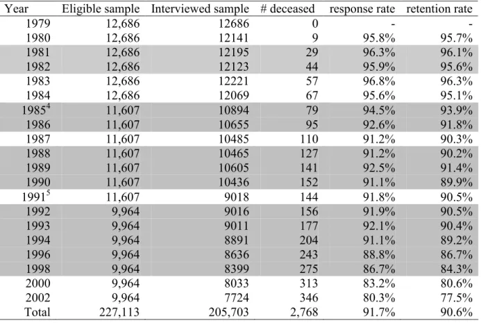
The NLSY79 has maintained a high retention rate over the survey years. Around 90% of the NLSY respondents remaining eligible for interview participated in the survey during the survey years. All base-year respondents, including those reported to be deceased, are considered eligible for interview except those who have been dropped from the sample (see Table 4.1).

(47)

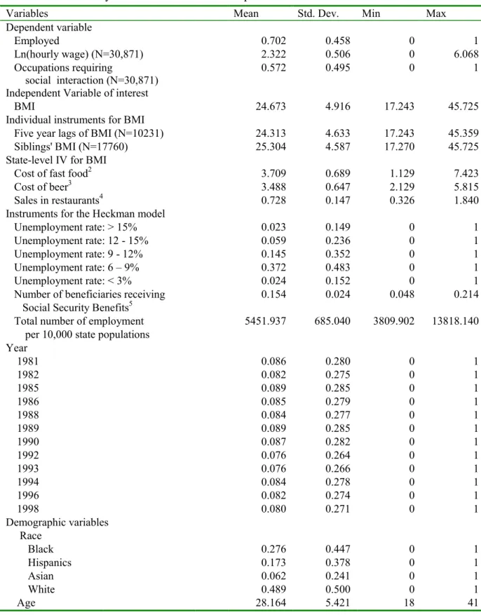
than 6 times in 12 interviews over 17 years; 6) upper or lower 1% of the overall distribution of BMI; and, 7) answered that health problems limited types or amount of works. Men and women are represented the final sample almost equally (47, 435 and 44,000 person-years, or 5,391 and 5,220 persons for men and women, respectively). Among those exclusion criteria, the number of person-year observations excluded due to their health problems limiting types or amount of works is 2,726 and 2,043 for men and women, respectively. Tables 4.2a and 4.2b show the overall distribution of the variables in the final sample by gender.

Dependent variables

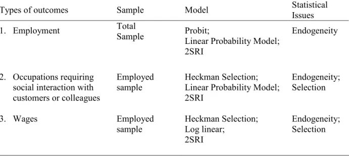
This study used three measures of labor market outcomes as the dependent variables: employment, occupation, and wage. Table 4.3 summarizes the types of outcomes in the labor markets as the dependent variables, samples, models, and several of the statistical issues to be anticipated.

Employment

As displayed in Table 4.4, the probability of employment was estimated for total samples within gender, while the other two measurements of dependent variables (the probability of occupation where social interaction with customers or colleagues is required, and wages) was estimated for employed samples within gender.

(48)

or businesses from which she was temporarily absent because of illness, bad weather, vacation, labor-management disputes, or various personal reasons, whether they were paid for the time off or were seeking other jobs” (NLSY79 User’s Guide, 2004). That is, any sample person out of the labor force except for temporary reasons was considered as unemployed in this study.

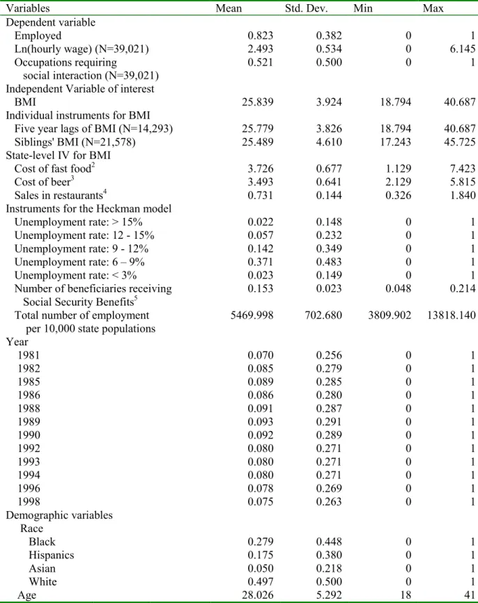
Men were employed slightly more than women in the final sample. Eighty two percent (39,021 years of 47,435 years) were employed, while 70% (30,871 person-years among 44,000 person-person-years) were employed.

Overall, men switched employment status either from employment to non-employment or vice versa less often than women (37.9% for men versus 41.2% for women) in the total sample. The proportion of the sample persons who ever changed the employment status from employment to non-employment was higher in women than men (26.4% for women versus 16.4% for men), while it was opposite in the cases for the sample persons who ever changed the employment status from non-employment to employment. This different pattern for the switch in the employment status may be related to child birth, following maternity leave, and child-rearing for women.

The proportion of the sample persons who ever switched their employment status in either direction was different by age groups: a higher proportion of men ever switched employment status than women for 18-24 age group, while the trend was opposite in the rest of the age groups (see table 4.4).

Wages

(49)

Having no wages may indicate that the wages those individuals could earn if they were to work were simply unobserved. Because non-working individuals with unobserved wages are likely to be systemically different than working individuals with observed positive wages, the Heckman selection model with controls for selection is appropriate (Puhani, 2000). The identifying instruments in the Heckman selection model included the following three state-level variables: unemployment rate, number of business establishments, and number of Social Security Program beneficiaries (Cawley, 2000; Puhani, 2000; MaCurdy, Green, and Paarsch, 1990).

The NLSY79 collected data on respondents’ usual earnings including tips, overtime, and bonuses but before deductions during every survey year for each employer for whom the respondent worked since the last interview date (NLSY79 User’s Guide, 2004). For this study, wages were measured by the hourly rate of pay at the most current or the most recent job (CPS job). Yearly inflation was adjusted in the hourly wages at the CPS job by GDP deflator. The hourly wages greater than $400 before adjusting for the GDP deflator were replaced as missing.

(50)

Occupations where social interaction with customers or colleagues is required

Like wages, occupations were observed only for people participating in the labor force. The difference in characteristics between working individuals and non-working individuals also applied to the estimation of the effect of obesity on the probability of having occupations where social interaction with customers or colleagues is required. Thus, the Heckman selection model was also be used to control for the selection in the measurement of occupations where social interaction with customers or colleagues is required. The identifying instruments in the Heckman selection model were the same as in the wages equation.

(51)

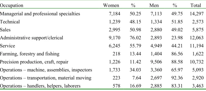
support/clerical category. Women also composed more than half in the service category. For the sales, and managerial and professional specialties, both genders had similar proportions (see Table 4.5).

(52)

codes. Around half of the employed population had occupations where social interaction with customers or colleagues is required in the final sample (52.03% for men and 56.39% for women).

In the NLSY79, occupations were coded following the Census 1980 until 1998. Census 1980 codes cannot be linked to the DOT codes directly. Thus, for this study, several linking algorithms were adopted for assigning the 5th digit of the DOT codes to each of the occupation codes in the final sample by matching the occupation code in the Census 1980 system in the data and the DOT codes. The DOT codes are linked to the Occupational Information Network (O*NET) codes by a matching algorithm provided by the developer of the O*NET system. O*NET is a comprehensive database of worker attributes and job characteristics, which was developed as the replacement for the DOT. The first edition of O*NET was released in 1998. O*NET codes can be linked to the Census 2000 codes by its original design. Also, the Census Bureau provides a matching table for linking occupation codes in the Census 2000 to the old Census including the 1980 Census. Through these multiple matching algorithms, the DOT codes and the occupation codes in the O*NET system were linked to the 1980 census occupation codes.

(53)

coordination, instructing, negotiation, persuasion, service orientation, and social perceptiveness (O*NET resource center, accessed in 2005). This study took the occupations that require those social skills as the occupations where slimness may reward performances in jobs. Therefore, a dummy variable representing occupations where social interaction with customers or colleagues is required was generated as a dependent variable for the occupations requiring social skills in the O*NET. The proportion of sample persons in the occupations where social interaction with customers or colleagues is required dropped to around one third when those occupations were identified using the O*NET system compared to the DOT codes (30.21% for women and 22.63% for men).

As a composite measure, a dummy variable was generated for characterizing occupations that were classified to require social interaction with customers or colleagues either in the DOT codes or O*NET system. As expected, the proportion of sample persons in occupations where social interaction with customers or colleagues is required increased in both genders compared to two different measures described above (62.23% women versus 70.20% for men). In the final analysis, only the composite measure of occupations was used.

(54)

both genders. A higher proportion of men ever switched occupations status than women for all age groups except the oldest 35-41 years of age group (see Table 4.6).

Explanatory Variables

The variable of primary interest is the extent of obesity, which was measured with body mass index (BMI). BMI is defined as weight in kilograms divided by height in meters squared. In the NLSY79, height (self-reported by the respondents) information was collected only three times, 1981, 1982, and 1985, although the respondent’s current weight (self-reported by the respondents) has been collected in every round of the survey. However, given that respondents were between 20 and 27 in 1985, height in 1985 was used as the respondents’ adult height on the assumption that height typically stops changing at those ages (Cawely, 2004).

(55)

height and weight in the NHANES III may be different from other survey with only self-reported height and weight like the NLSY79.

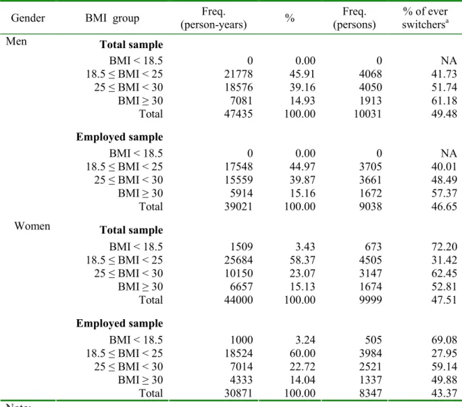
Persons with BMI equal to or greater than 30 are classified as obese. A BMI between 25 and 30 is classified as overweight, and BMI below 18.5 is underweight (National Heart, Lung, and Blood Institute, 1998). Four BMI splines were generated with cut points 18.5, 25, and 30 to obtain the different marginal effect of BMI on each category of state of being obese on labor market outcomes.

BMI in the total sample increased over time as sample persons aged for both genders. This increase in BMI over ages also was clear when BMI were categorized into the four groups as described above. The proportion of being overweight and obese increased over age while the proportion of the normal weight declined over age for both genders (see figure 4.1 and 4.2).

(56)

diverged from 12% to 52% (see Table 4.8a and 4.8b). In another measure of within person and between persons variations of BMI, the continuous BMI per person was decomposed into the mean of BMI over time per person and the deviations of BMI of a person in each time from the average BMI over time per person. The standard deviation of those two components of BMI was displayed in Table 4.9 for the total and employed sample by men and women. Overall, average BMI varied between 17 and 45. Deviation of BMI at time t for each sample person ranged -18 and 15. Within person variation in BMI over time was more than half of the variation in BMI across sample persons in both the total and employed sample for both genders (see Table 4.9).

Other descriptive data distributions

The proportion of sample persons with a college or higher education was greater for women than men across ages over 25. For example, at age 30, around 30 to 34% of the sample had obtained college or higher education. Overall, up to 33 to 37% in the total sample received college or higher education (see Table 4.9).

In Table 4.10a and 4.10b, Hispanic Whites were 49% of the total sample, and non-Hispanic Blacks were 28%. non-Hispanic and Asian had a smaller proportion, which composed 17% and 6%, respectively, of the final sample. Among four regional areas inclusive of Northeast, North-central, South, and West, sample persons in South were 39% of the total sample, while the other three regional areas were composed almost evenly (18% in Northeast, 24% in North-central, and 19% in South).

(57)

(58)

Table 4.1 Sample sizes, retention rates, and response rates in the NLSY79

Year Eligible sample Interviewed sample # deceased response rate retention rate

1979 12,686 12686 0 - -

1980 12,686 12141 9 95.8% 95.7%

1981 12,686 12195 29 96.3% 96.1%

1982 12,686 12123 44 95.9% 95.6%

1983 12,686 12221 57 96.8% 96.3%

1984 12,686 12069 67 95.6% 95.1%

19854 11,607 10894 79 94.5% 93.9%

1986 11,607 10655 95 92.6% 91.8%

1987 11,607 10485 110 91.2% 90.3%

1988 11,607 10465 127 91.2% 90.2%

1989 11,607 10605 141 92.5% 91.4%

1990 11,607 10436 152 91.1% 89.9%

19915 11,607 9018 144 91.8% 90.5%

1992 9,964 9016 156 91.9% 90.5%

1993 9,964 9011 177 92.1% 90.4%

1994 9,964 8891 204 91.1% 89.2%

1996 9,964 8636 243 88.8% 86.7%

1998 9,964 8399 275 86.7% 84.3%

2000 9,964 8033 313 83.2% 80.6%

2002 9,964 7724 346 80.3% 77.5%

Total 227,113 205,703 2,768 91.7% 90.6%

Notes:

1. Source: NLSY79 User’s Guide: A Guide to the 1979–2002 National Longitudinal Survey of Youth Data.

2. Response rate is defined as “the percentage of base-year respondents remaining eligible and not known to be deceased who were interviewed in a given survey year”.

3. Retention rate is calculated by “dividing the number of respondents interviewed by the number of respondents remaining eligible for interview.” All 1979 (round 1) respondents including those reported as deceased are eligible for interviews, with the exception of those who have been permanently dropped from the sample.

4. After the 1984 surveys, interviewing ceased for 1,079 members of the military sub-sample; retained for continued interviewing were 201 respondents randomly selected from the original entire military sample of 1,280; 186 of the 201 participated in the 1985 interview. The total number of the NLSY79 civilian and military respondents eligible for interview (including deceased respondents) beginning in 1985 was 11,607.

5. The 1,643 economically disadvantaged non-Black/non-Hispanic men and women members of the supplemental sub-sample were not eligible for interview as of the 1991 survey year. The total number of the NLSY79 civilian and military respondents eligible for interview (including deceased respondents) beginning in 1991 was 9,964.

(59)

Table 4.2a Summary statistics for the final sample: women1

Variables Mean Std. Dev. Min Max

Dependent variable

Employed 0.702 0.458 0 1

Ln(hourly wage) (N=30,871) 2.322 0.506 0 6.068

Occupations requiring

social interaction (N=30,871)

0.572 0.495 0 1

Independent Variable of interest

BMI 24.673 4.916 17.243 45.725

Individual instruments for BMI

Five year lags of BMI (N=10231) 24.313 4.633 17.243 45.359

Siblings' BMI (N=17760) 25.304 4.587 17.270 45.725

State-level IV for BMI

Cost of fast food2 3.709 0.689 1.129 7.423

Cost of beer3 3.488 0.647 2.129 5.815

Sales in restaurants4 0.728 0.147 0.326 1.840

Instruments for the Heckman model

Unemployment rate: > 15% 0.023 0.149 0 1

Unemployment rate: 12 - 15% 0.059 0.236 0 1

Unemployment rate: 9 - 12% 0.145 0.352 0 1

Unemployment rate: 6 – 9% 0.372 0.483 0 1

Unemployment rate: < 3% 0.024 0.152 0 1

Number of beneficiaries receiving 0.154 0.024 0.048 0.214

Social Security Benefits5

Total number of employment 5451.937 685.040 3809.902 13818.140

per 10,000 state populations Year

1981 0.086 0.280 0 1

1982 0.082 0.275 0 1

1985 0.089 0.285 0 1

1986 0.085 0.279 0 1

1988 0.084 0.277 0 1

1989 0.089 0.285 0 1

1990 0.087 0.282 0 1

1992 0.076 0.264 0 1

1993 0.076 0.266 0 1

1994 0.084 0.278 0 1

1996 0.082 0.274 0 1

1998 0.080 0.271 0 1

Demographic variables Race

Black 0.276 0.447 0 1

Hispanics 0.173 0.378 0 1

Asian 0.062 0.241 0 1

White 0.489 0.500 0 1

(60)

Table 4.2a Summary statistics for the final sample: women – continued

Variables Mean Std. Dev. Min Max

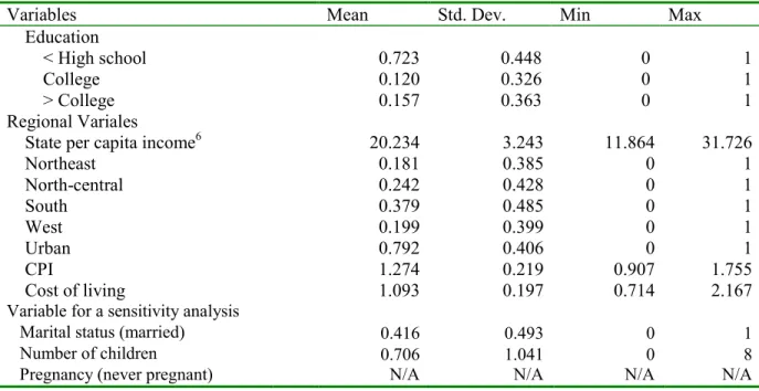
Education

< High school 0.684 0.465 0 1

College 0.152 0.359 0 1

> College 0.164 0.370 0 1

Regional Variables

State per capita income6 20.134 3.316 11.864 31.726

Northeast 0.177 0.382 0 1

North-central 0.230 0.421 0 1

South 0.407 0.491 0 1

West 0.185 0.389 0 1

Urban 0.788 0.409 0 1

CPI 1.273 0.224 0.907 1.755

Cost of living 1.086 0.188 0.714 2.167

Variable for a sensitivity analysis

Marital status (married) 0.453 0.498 0 1

Number of children 1.098 1.188 0 9

Pregnancy (never pregnant) 0.448 0.497 0 1

Notes:

1. Total observations are 44,000 unless otherwise noted.

2. Average cost of the following three items: a McDonald’s Quarter-Pounder with cheese, a thin crusted cheese pizza at Pizza Hut or Pizza Inn, fried chicken at Kentucky Fried Chicken or Church’s (Chou, Grossman, and Saffer, 2002).

3. Average price of a bottle of Budweiser Schlitz before the fourth quarter of 1989, and Budweiser and Miller Light as of the fourth quarter of 1989.

(61)

Table 4.2b Summary statistics for the final sample: men1

Variables Mean Std. Dev. Min Max Dependent variable

Employed 0.823 0.382 0 1

Ln(hourly wage) (N=39,021) 2.493 0.534 0 6.145 Occupations requiring

social interaction (N=39,021)

0.521 0.500 0 1 Independent Variable of interest

BMI 25.839 3.924 18.794 40.687 Individual instruments for BMI

Five year lags of BMI (N=14,293) 25.779 3.826 18.794 40.687 Siblings' BMI (N=21,578) 25.489 4.610 17.243 45.725 State-level IV for BMI

Cost of fast food2 3.726 0.677 1.129 7.423 Cost of beer3 3.493 0.641 2.129 5.815 Sales in restaurants4 0.731 0.144 0.326 1.840 Instruments for the Heckman model

Unemployment rate: > 15% 0.022 0.148 0 1 Unemployment rate: 12 - 15% 0.057 0.232 0 1 Unemployment rate: 9 - 12% 0.142 0.349 0 1 Unemployment rate: 6 – 9% 0.371 0.483 0 1 Unemployment rate: < 3% 0.023 0.149 0 1 Number of beneficiaries receiving 0.153 0.023 0.048 0.214 Social Security Benefits5

Total number of employment 5469.998 702.680 3809.902 13818.140 per 10,000 state populations

Year

1981 0.070 0.256 0 1

1982 0.085 0.279 0 1

1985 0.089 0.285 0 1

1986 0.086 0.280 0 1

1988 0.091 0.287 0 1

1989 0.093 0.291 0 1

1990 0.092 0.289 0 1

1992 0.080 0.271 0 1

1993 0.080 0.271 0 1

1994 0.080 0.271 0 1